“All structures, properly understood, from the solar system to the atom, are tensegrity structures. Universe is omnitensional integrity”
—R. Buckminster Fuller, Synergetics, 700.04

All structures, from the quantum to the cosmological, consist of islands of compression held together by a continuous web of tension. Continuous surfaces and solids are emergent properties of scale. At cosmological scales, the islands of compression are clusters of matter—dust clouds, planets, galaxies, etc.— in which inertial forces (and, perhaps, something called “dark energy”) provide the resistance in opposition to universal gravitation, the continuous web of tension that is mass attraction. At the microscopic level, the islands of compression are atoms and molecules in which radiant energy provides compressive resistance against the electromagnetic and nuclear forces providing the continuous web of tension that binds molecules and atoms together.

Gravity and inertia, the electromagnetic force and electromagnetic radiation, and tension and compression are all as inseparable from one another as the the push and pull of steel spring. Each pair, though often presented as fundamentally distinct phenomena, are really two views of the same thing, like the convex and concave surfaces of the sphere.

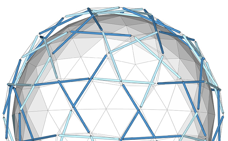
“Tensegrity” is a portmanteau of tension and integrity. It refers to standalone structures that would have as much integrity in the vacuum of space as on the earth’s surface. In its purest form, a tensegrity structure consists of isolated rigid elements, struts, suspended in an unbroken web of tension, tendons. Fuller’s geodesic domes constitute a special case of tensegrities, which constitute the more general class, and the way to an intuitive understanding of geodesic domes is to understand tensegrities first.

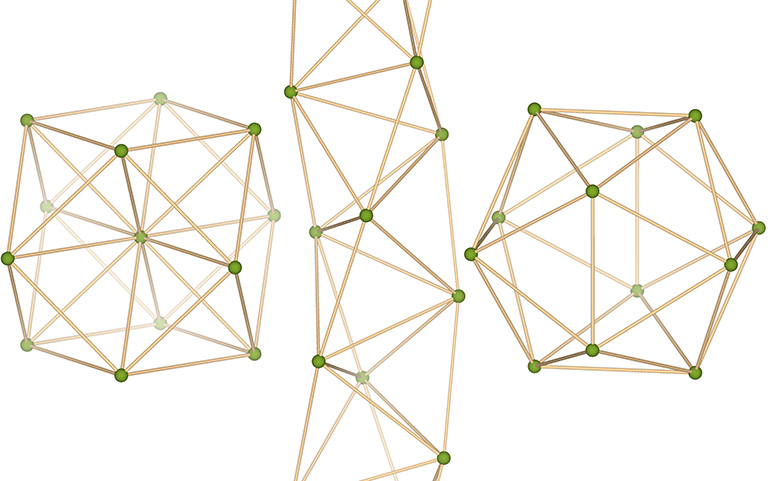
The three basic structural polyhedra, the tetrahedron, octahedron, and icosahedron, can be constructed using these principles. The struts comprising their edges do not touch, but are held in place by the tendons that form a continuous tension web.

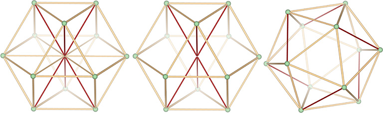
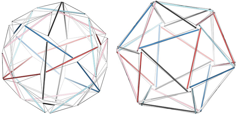
Though perhaps not immediately apparent, the three tensegrity polyhedra are transformations of the three tensegrity spheres; the 6-strut Jessen icosahedron, the 12-strut cuboctahedron, and the 30-strut icosidodecahedron.

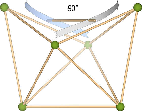
The transformation involves the clockwise or counter-clockwise torque of the struts. All transformations between the spherical and polyhedral phases are stable. However, the 12- and 30-strut tensegrities are configured as either right- or left-handed and will transform in one direction only. Only the 6-strut tensegrity is ambidextrous; the same spherical condition transforms into either a positive or a negative (right- or left-handed) tetrahedron depending on whether the struts are torqued to the right or to the left. This is in keeping with the unique duality of the tetrahedron. See: The Dual Nature of the Tetrahedron.

The struts of the three spherical tensegrities are arranged in a pattern of intersecting great circles, or geodesics, each of which divide the sphere into two equal halves: the six-strut tensegrity sphere consists of three intersecting great circle rings of two struts each; the twelve-strut spherical tensegrity consists of four great circle rings of three struts each; and the thirty-strut tensegrity consists of six intersecting great circle rings of five struts each.

This suggests an alternative construction of the tensegrity spheres that has the great circles forming discrete tension loops with the tendons emerging from the strut ends and passing directly under (or through) the cross struts, or “danglers”. The great circles intersect in a stable basket-weave pattern. This strut-and-sling alternative emphasizes the equilibrium state of the spherical tensegrities, as opposed to their more disequibrious, semi-polyhedron states. See: Tensegrity Equilibrium and Vector Equilibrium.

In the transformation from tensegrity sphere to polyhedron, the struts forming the great circles diverge along the path of their danglers. Their paths encircle the polyhedron in zigzag patterns that constitute a geodesic or equatorial “wave” consisting of the primary struts and their danglers.

Note that the great circles of the 12- and 30-strut tensegrities incorporate one dangler each from all of the other great circles. That is, all their great circles intersect each of the others. The great circles of six-strut tensegrity, however, are unique; the struts from only one of the two other great circles serve as danglers in any given great circle. That is, each great circle incorporates all the struts from two and none from the third. This, again, points to the dual nature of the tetrahedron.

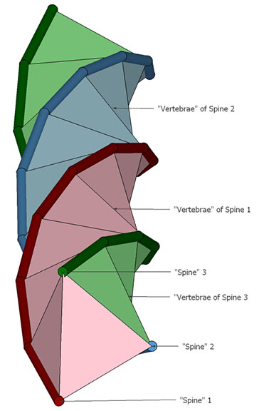
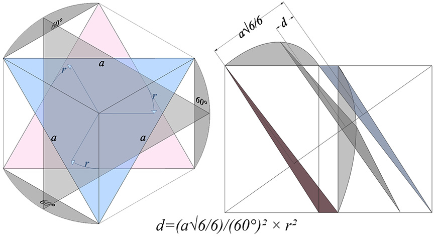
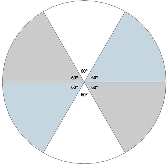
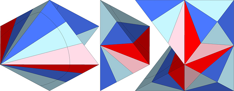
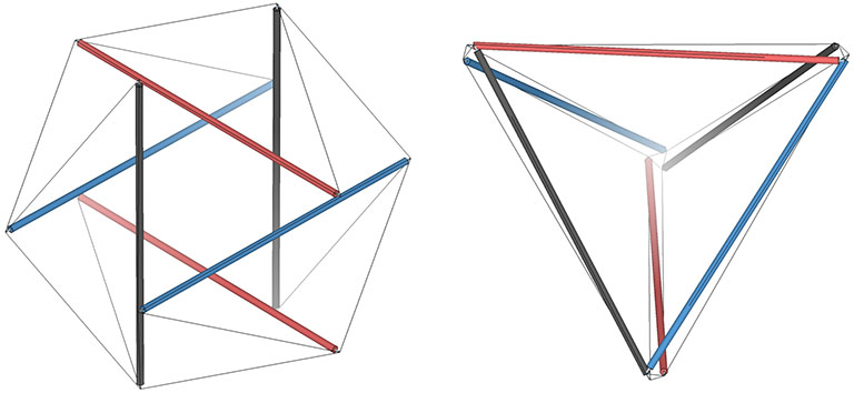
In the figure below, the three great circles of the six-strut tensegrity sphere are arranged as follows in its tetrahedron counterpart:

1. red-blue-red-blue (red great circle incorporates only blue danglers);
2. blue-black-blue-black (the blue great circle incorporates only black danglers);
3. black-red-black-red (the black great circle incorporates only red danglers).

The four great circles of the twelve-strut tensegrity incorporate struts from each of the others to form six-strut equatorial bands around the face-to-face poles of the octahedron. Note that the four-strut equatorial bands of the octahedron’s three vertex-to-vertex poles incorporate one strut each from all four great circles.

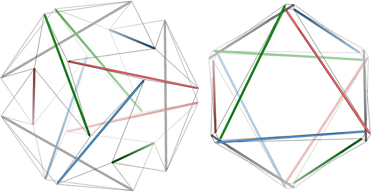
In the figure below, the four great circles of the 12-strut tensegrity sphere are arranged as follows in its octahedron counterpart:

1. red-gray-red-blue-red-green
2. blue-red-blue-green-blue-gray
3. green-blue-green-red-green-gray
4. gray-blue-gray-green-gray-red

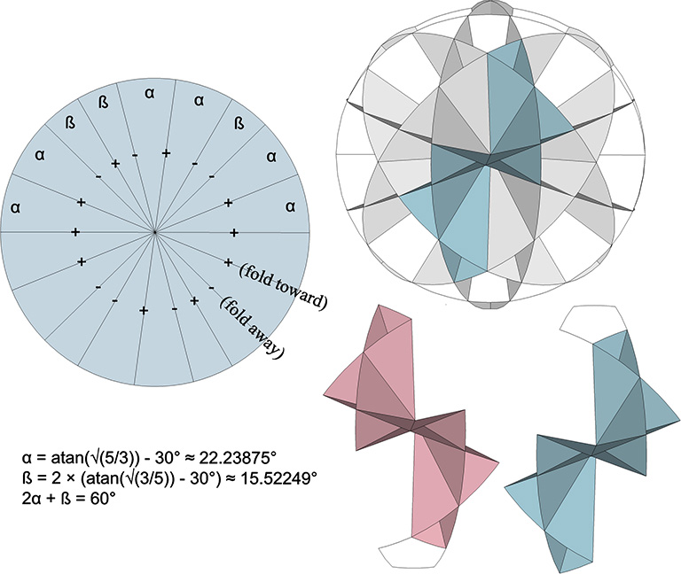
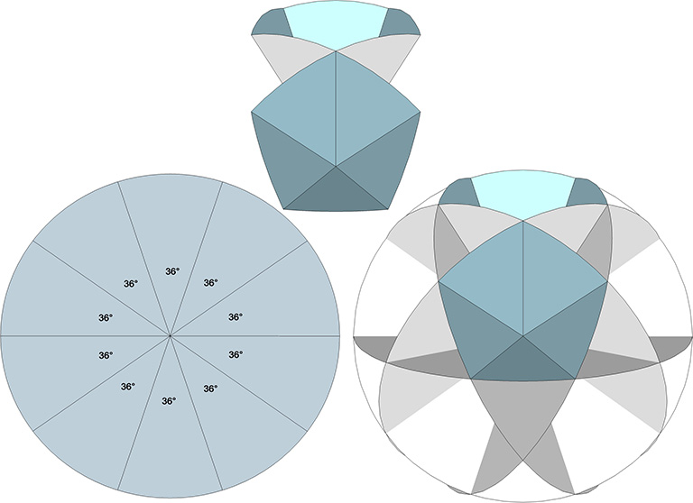
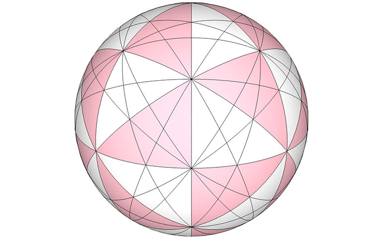
The six great circles of the thirty-strut tensegrity incorporate struts from each of the others to form ten-strut equatorial bands around the vertex-to-vertex poles of the icosahedron. Note that six-strut equatorial bands of the icosahedron’s five face-to-face poles incorporate one strut each from all six great circles.

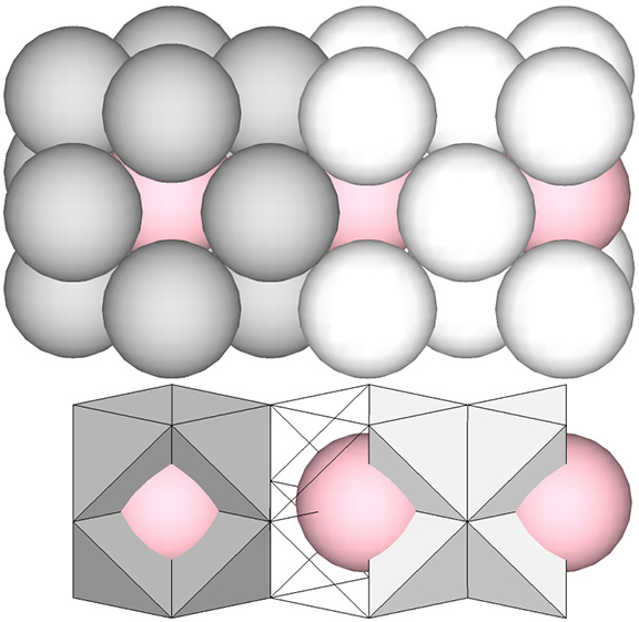
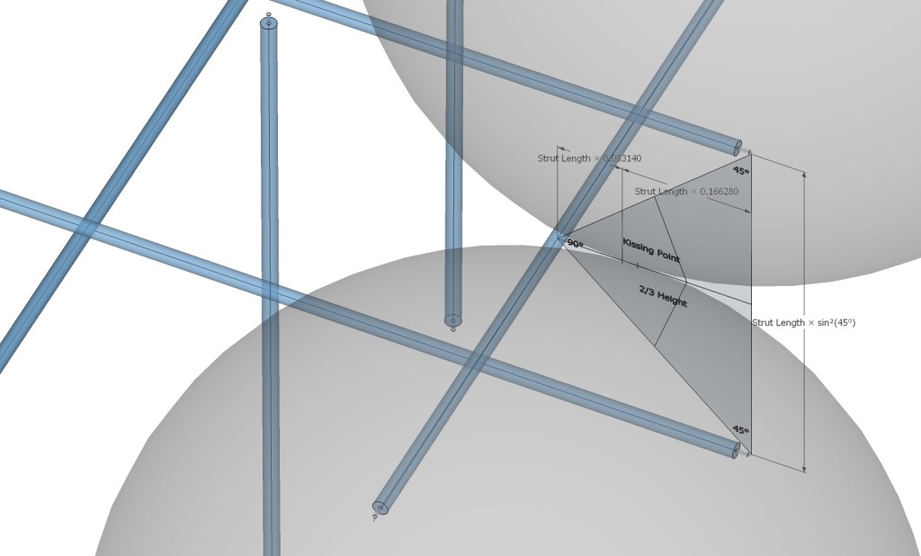
The spherical tensegrities relate to the close packing of spheres. In their “relaxed” states, the strut ends straddle the points of contact between the spheres, what Fuller called the “kissing points.” The kissing points lie on the plane connecting the midpoint of the dangler with the endpoints of its two supporting struts.

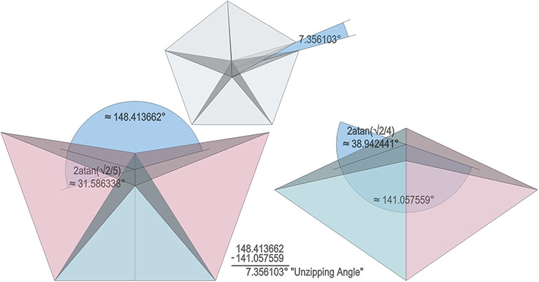
In the 12-strut tensegrity, this forms an equilateral triangle whose base edge length (the distance between the supporting struts’ endpoints) equals the strut length multiplied by sin²(30°), or 0.25. The distance from the midpoint of the dangler to the kissing point is approximately 0.066987 times the strut length.

In the 30-strut tensegrity, this forms an 36° 72° 72° isosceles triangle whose base edge length (the distance between the supporting struts’ endpoints) equals the strut length multiplied by sin²(18°), or about 0.095492. The distance from the midpoint of the dangler to the kissing point is approximately 0.03956 times the strut length.

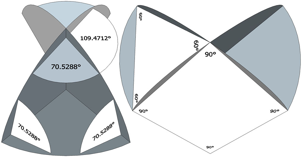
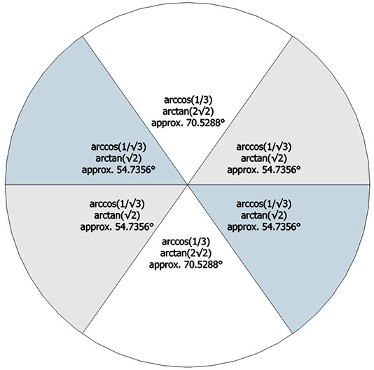
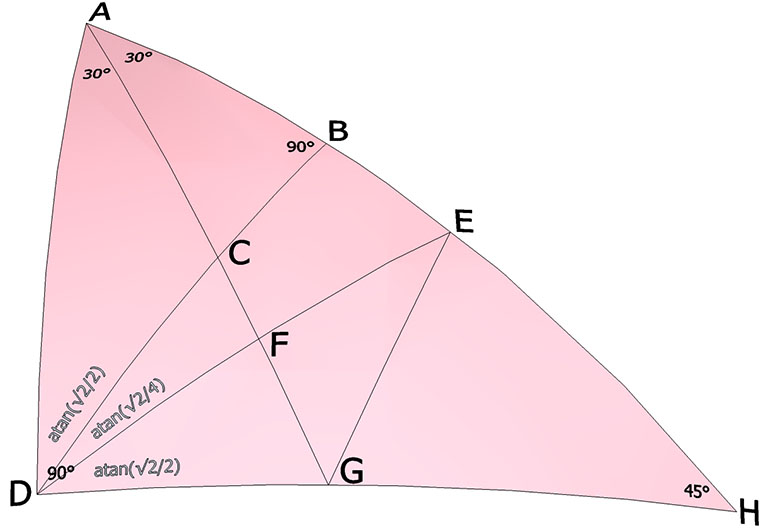
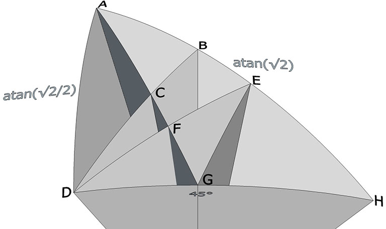
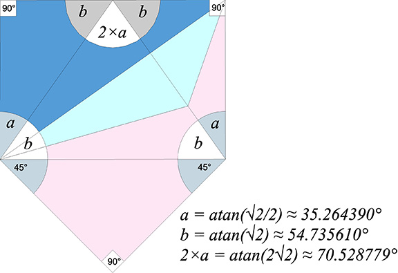
In the 6-strut tensegrity, this forms an 90° 45° 45° isosceles triangle whose base edge length (the distance between the supporting struts’ endpoints) equals the strut length multiplied by sin²(45°), or 0.5. The distance from the midpoint of the dangler to the kissing point is approximately 0.083140 times the strut length.

In their polyhedron states, the strut ends approach the sphere centers. In the twelve-strut tensegrity, the strut ends move from the kissing points to the centers of the six spheres defining the octahedron:

In the thirty-strut tensegrity, the strut ends move from the kissing points to the centers of the twelve spheres defining the icosahedron:

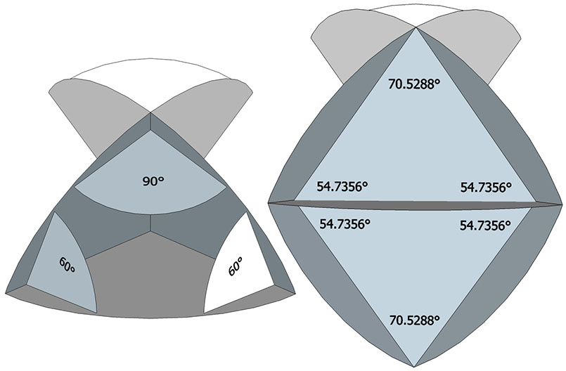
In the six-strut tensegrity, the strut ends move from the kissing points to the centers of the six spheres defining the tetrahedron. Because the six-strut tensegrity can be twisted to form either a positive or a negative tetrahedron, it can oscillate between the two in an uninterrupted transformation.

This unique ability of the tetrahedron to turn itself inside out provides another model of the the sphere-to-space, space-to-sphere oscillations of the jitterbug. If we replace the tetrahedra in the vector model with the six-strut tensegrity, its oscillations between the positive and the negative tetrahedron alternately define the nuclear sphere at the the center of the VE, and the concave VE at the center of the octahedron.

Sphere centers and interstices are identified by tendon loops in the spherical tensegrities. In the figure below, the red polygonal (square) loops of the relaxed 12-strut tensegrity are coincident with the sphere centers, and the yellow triangular loops are coincident with the interstices. See Spheres and Spaces.

If we apply a counter-clockwise torque to a clockwise (and vice versa) 12-strut tensegrity, we force the tensegrity into the unstable* configuration of the cube.

The counter-clockwise torque of a clockwise (and vice versa) 30-strut tensegrity forces it into the unstable* configuration of the pentagonal dodecahedron. Because the 12- and 30-strut tensegrities must always and only be either right- or left-handed, and never both simultaneously, nature disallows these operations.

* “Unstable” may be too strong a word. The tensegrities of otherwise non-rigid (i.e., non-triangulated) polyhedra, like the cube and the pentagonal dodecahedron do hold their shape. However, their strength decreases as the diameter of their vertex loops shrink to points.

Fuller described tensegrities as balloons evacuated of all the supporting gas except for those molecules actively careening around the inside surface on trajectories that are the chords of geodesics. The underlying structure is disclosed by replacing those careening molecules with static struts, and then removing all of the balloon’s skin except for a continuous web of tensile fibers holding the struts in place. A very high frequency tensegrity sphere with all redundancy and non-essential components removed could, in theory, be reduced to molecular bonds, atomic bonds, and ultimately disappear entirely into highly organized quantum fields.

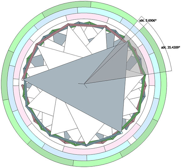
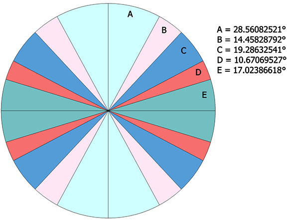
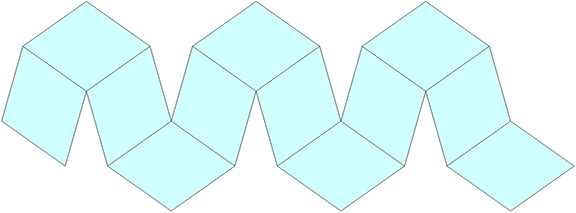
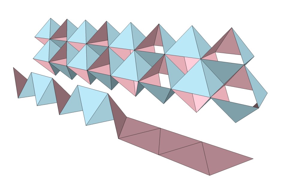
There is another class of tensegrities commonly called tensegrity prisms. The simplest in this class consists of three struts and nine tendons, and has the shape of a triangular prism with the top triangle twisted at 30° from the bottom triangle. Any number of tensegrity prisms are possible. Each is defined by the number of struts which corresponds to the number of sides in the polygon on which is based. In the figure below are tensegrity prisms based on polygons with 3, 4, 5, 6, and 10 sides.

The angle at which the top polygon is twisted in relation to the bottom polygon is a constant and is given by the formula,

90°-(180°/n)

where n is the number of struts, or sides of the polygon on which it is based.

Tensegrity prisms have been combined to form columns, lattices, and complex hyperbolic surfaces. They have also been employed in multi-layered geodesic domes. The possibilities are practically unlimited.

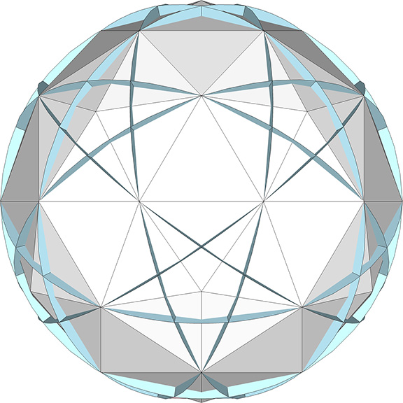
Though building codes assessed Fuller’s geodesic domes as conventional truss networks, they were designed and engineered as tensegrity structures. Redundancies were then added to please the inspectors, and to satisfy the clients’ desire for something that looked substantial. Most were based on the icosahedron, with the 30-strut tensegrity sphere serving as the base model. Regular, triangular subdivisions of the icosahedron create the primary faces of the geodesic polyhedra, all of which (if based on the icosahedron) will have 12 vertices with 5 members, and a larger number of vertices with 6 members. In the spherical tensegrities, these form tension loops of pentagons and hexagons.

All the spherical tensegrities can be reduced to geodesic polyhedra. If we draw in to a point the pentagonal and hexagonal loops in the 120-strut tensegrity sphere above, its 80 triangles enlarge to form the 2F Class 1 geodesic polyhedron.

As frequency and the number of struts increases in the spherical tensegrities, the distance between the struts decreases and the tension and compression elements begin to merge in accordance with the following identities:

dig angle (Φ) = 180°/n
gap = sin²(Φ/2)
dip= 1/2 × sin(Φ/2)

where n = the number of sides in the great (or lesser) circle being assessed. It is the case with most of Fuller’s geodesic domes that the tension web runs through the struts and is therefore implied rather than explicit.

Fuller saw great engineering potential in the understanding of structure as tensegrity:

“As the world’s high-performance metallic technologies are freed from concentration on armaments, their structural and mechanical and chemical performances (together with the electrodynamic remote control of systems in general) will permit dimensional exquisiteness of mass-production-forming tolerances to be reduced to an accuracy of one-hundredth-thousandths of an inch. This fine tolerance will permit the use of hydraulically pressure-filled glands of high-tensile metallic tubing using liquids that are nonfreezable at space-program temperature ranges, to act when pressurized as the discontinuously isolated compressional struts of large geodesic tensegrity spheres. Since the fitting tolerances will be less than the size of the liquid molecules, there will be no leakage. This will obviate the collapsibility of the air-lock-and-pressure- maintained pneumatic domes that require continuous pump-pressurizing to avoid being drag-rotated to flatten like a candle flame in a hurricane. Hydro-compressed tensegrities are less vulnerable as liquids are noncompressible.

“Geodesic tensegrity spheres may be produced at enormous city-enclosing diameters. They may be assembled by helicopters with great economy. This will reduce the investment of metals in large tensegrity structures to a small fraction of the metals invested in geodesic structures of the past. It will be possible to produce geodesic domes of enormous diameters to cover whole communities with a relatively minor investment of structural materials. With the combined capabilities of mass production and aerospace technology it becomes feasible to turn out whole rolls of noncorrosive, flexible-cable networks with high-tensile, interswaged fittings to be manufactured in one gossamer piece, like a great fishing net whose whole unitary tension system can be air-delivered anywhere to be compression-strutted by swift local insertions of remote-controlled, expandable hydro-struts, which, as the spheric structure takes shape, may be hydro-pumped to firm completion by radio control.

“In the advanced-space-structures research program it has been discovered that—in the absence of unidirectional gravity and atmosphere—it is highly feasible to centrifugally spin-open spherical or cylindrical structures in such a manner that if one-half of the spherical net is prepacked by folding below the equator and being tucked back into the other and outer half to form a dome within a dome when spun open, it is possible to produce domes that are miles in diameter. When such structures consist at the outset of only gossamer, high-tensile, low-weight, spider-web-diameter filaments, and when the spheres spun open can hold their shape unchallenged by gravity, then all the filaments’ local molecules could be chemically activated to produce local monomer tubes interconnecting the network joints, which could be hydraulically expanded to form an omniintertrussed double dome. Such a dome could then be retrorocketed to subside deceleratingly into the Earth’s atmosphere, within which it will lower only slowly, due to its extremely low comprehensive specific gravity and its vast webbing surface, permitting it to be aimingly-landed slowly, very much like an air-floatable dandelion seed ball: the multi-mile-diametered tensegrity dome would seem to be a giant cousin. Such a space- spun, Earth-landed structure could then be further fortified locally by the insertion of larger hydro-struttings from helicopters or rigid lighter-than-air- ships—or even by remote-control electroplating, employing the atmosphere as an electrolyte. It would also be feasible to expand large dome networks progressively from the assembly of smaller pneumatic and surface-skinning components.

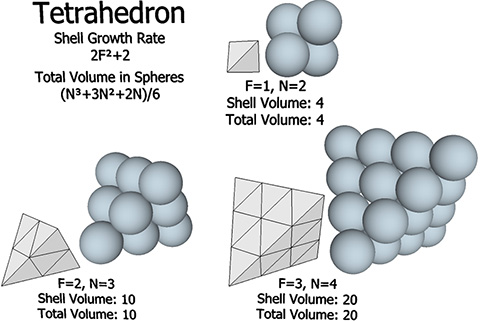
“The fact that the dome volume increases exponentially at a third-power rate, while the structural component lengths increase at only a fraction more than an arithmetical rate, means that their air volume is so great in comparison to the enclosing skin that its inside atmosphere temperature would remain approximately tropically constant independent of outside weather variations. A dome in this vast scale would also be structurally fail-safe in that the amount of air inside would take months to be evacuated should any air vehicle smash through its upper structure or break any of its trussing.

“In air-floatable dome systems metals will be used exclusively in tension, and all compression will be furnished by the tensionally contained, antifreeze-treated liquids. Metals with tensile strengths of a million p.s.i. will be balance-opposed structurally by liquids that will remain noncompressible even at a million p.s.i. Complete shock-load absorption will be provided by the highly compressible gas molecules—interpermeating the hydraulic molecules—to provide symmetrical distribution of all forces. The hydraulic compressive forces will be evenly distributed outwardly to the tension skins of the individual struts and thence even further to the comprehensive metal- or glass-skinned hydro-glands of the spheroidally enclosed, concentrically-trussed-together, dome-within-dome foldback, omnitriangulated, nonredundant, tensegrity network structural system.“
—R. Buckminster Fuller, Synergetics, sections 785.03-07, (1975)

“These helical columns of tetrahedra, which we call the tetrahelix, explain the structuring of DNA models of the control of the fundamental patterning of nature’s biological structuring as contained within the virus nucleus. It takes just 10 triple-bonded tetrahedra to make a helix cycle, which is a molecular compounding characteristic also of the Watson-Crick model of the DNA. When we address two or more positive (or two or more negative) tetrahelices together, they nestle their angling forms into one another. When so nestled the tetrahedra are grouped in local clusters of five tetrahedra around a transverse axis in the tetrahelix nestling columns. Because the dihedral angles of five tetrahedra are 7° 20′ short of 360°, this 7° 20′ is sprung-closed by the helix structure’s spring contraction. This backed-up spring tries constantly to unzip one nestling tetrahedron from the other, or others, of which it is a true replica. These are direct (theoretical) explanations of otherwise as yet unexplained behavior of the DNA.”
—R. Buckminster Fuller, Synergetics, caption to fig. 933.01

Regular tetrahedra do not combine to fill all space. They can however be face-bonded to form a helical structure Fuller called the “tetrahelix.”

The tetrahelix can be constructed as a single, double, or triple helix, oriented either clockwise or counter-clockwise. The single helix completes about 10 cycles per 30 tetrahedra; the double helix completes about 5, and the triple helix completes about 1 cycle per 30 tetrahedra.

The single helix is folded from a ribbon of equilateral triangles, with alternating folds in the same direction of 2arctan(√2/4) ≈ 38.931629° and 2arctan(√2) ≈ 109.471221°.

The double helix is folded from 2-panel-wide ribbon. The two panels are folded inward at 2arctan(√2/4) ≈ 38.931629°, and the individual triangles are folded in an alternating pattern of 2arctan(√2/5) ≈ 31.586338° away, and 2arctan(√2) ≈ 109.471221° away.

The triple helix is folded from 3-panel-wide ribbon. Each panel is folded the length of the ribbon at 2arctan(√2) ≈ 109.471221°. The individual triangles are folded in an alternating pattern of 2arctan(√2/4) ≈ 38.931629° away, and 2arctan(√2/5) ≈ 31.586338° toward.

A casual assessment of the triple helix might lead to the assumption that the two angles between which the three helices oscillate, i.e are folded in a repeating pattern of one fold up, and one fold down, etc., are the same angle. They are not. As a consequence, one tetrahelix cannot be nested with another. There is always a gap of approximately 7.356103°, which causes them to spring apart. Fuller called this gap the “unzipping angle”, and thought it might explain the behavior of replicating DNA molecules.

The models of the tetrahelix so far discussed are constructions that result in only the outer shell of the tetrahelix, i.e., a hollow tube with no interior faces. The interior faces can be folded from a separate strip. In the illustration below, two strips of triangles are folded and combined as a double helix that constitutes the surface of the tetrahelix, and a third strip of triangles is folded to constitute its internal structure. The third strip which is enclosed by the other two is is folded at angles of arctan(2√2) ≈ 70.528779° alternately toward and away. Its striking similarity to the structure of the DNA molecule, i.e. a double helix with paired connections, was not lost on Fuller.

The helical axis does not pass through through the center of volume of any of its constituent tetrahedra. With the edge length taken as unity, the spin axis of the tetrahelix crosses an edge-to-edge axis of each tetrahedron perpendicularly at a distance of √2/10 from its center of volume, and is tilted at an angle of arctan(1/2), about 26.565051°.

The point at which all possible spin axes pass through the tetrahedron’s faces appears to be precisely arctan(√2)/5, or about 10.947122° off-center along lines drawn from a vertex to the midpoint of the opposite edge. Their points of intersection form an equilateral triangle centered on the face with edge length 1/10th that of the face.

Each tetrahedron is rotated about the helical axis at an angle of arctan(2/√5)+90°, or arccos(-2/3), about 131.810315°, from the one below it. Every third tetrahedron constitutes a “vertebra” of one of the three “spines” of the tetrahelix.

Curiously, the number of tetrahedra is not rationally commensurable with the helical cycle. The helix appears to complete one cycle every 30 tetrahedra, but careful measurement shows the rotation to be just short of 360°. Each vertebra is rotated at an angle of 3arctan(2/√5) – 90°, about 35.430945° from the previous. Ten vertebrae almost, but not quite, complete one 360° cycle. With r being the rotation per vertebra, the difference is 360-(10r) ≈ 5.690553°.

One might assume that one and only one helix may be formed from each of the four faces of the tetrahedron, i.e., that there are four (4) possible helical constructions. Further consideration may allow for clockwise and counter-clockwise helices, making for a total of eight (8) possibilities. Actually, there are twelve (12) unique axes upon which the helix can be constructed.

Each of the twelve axes can be illustrated with a cube placed inside a regular tetrahedron and sized such that four of its eight corners intersect the four faces of the tetrahedron as an equilateral triangle of edge length 1/10th that of the tetrahedron. Each of the twelve axes is described by lines connecting the vertices of the triangle with the center of the cube’s face with which it intersects.

The twelve unique helices alternate between clockwise and counter-clockwise constructions.

Given the fact that the number of tetrahedra is incommensurate with helical cycle, and the fact that its angles are all individually and mutually irrational, the number of configurations possible from serial inside-outing of tetrahedra, including the number of possible orientations of the individual tetrahedra in a fixed coordinate system, may be infinite.

“The XYZ-rectilinear coordinate system of humans fails to accommodate any finite resolution of any physically experienced challenge to comprehension. Physical experience demonstrates that individual-unit wavelength or frequency events close-pack in spherical agglomerations of unit radius spheres.”
—R. Buckminster Fuller, Synergetics, 260.31

Unit-radius spheres close pack in three fundamentally different ways:

1. radially around a central nucleus to form the isotropic vector matrix;
2. laterally as discrete icosahedron shells and lattices (see The Icosahedron; and Close Packing of Icosahedra), and;
3. linearly as discrete triple helices of face-bonded tetrahedra (see Tetrahelix).

The relative stability of these arrangements is perhaps made more clear when modeled with unit-length sticks, representing the vectors connecting sphere centers, and flexible connectors. The radial array on the left is the vector equilibrium (VE) and isotropic vector matrix; the linear array in the middle is the tetrahelix; and the lateral array on the right is the icosahedral shell.

The transformation between the isotropic radial array and the linear (helical) array can be described as three face-bonded tetrahedra transforming into a single octahedron.

The structural transformation is more clearly illustrated with a vector model.

Fuller thought this transformation modeled quantum energy dispersion and absorption, with the three-tetrahedron array gaining one quantum of energy in the transformation to the octahedron, which has volume for four (3+1) tetrahedra. Likewise, the octahedron loses one quantum in the transformation from a volume of four to the volume of three tetrahedra.

Note that the transformation involves the 90° rotation of one of the struts. Fuller would identify this as an example of “precession” about which he had much to say. It occurred to him that whenever energy is gained, lost, or otherwise transformed by a system, precession is always involved, and is geometrically manifested in effects at 90° to the perceived action.

The transformation between the radial and the lateral can be described as the transformation that occurs when the nuclear sphere is removed from the VE configuration. The twelve remaining spheres then rearrange themselves into an icosahedron.

The VE twists to the right or to the left to form a positive or a negative icosahedron. Note that this effect, too, is precessional, i.e., the gain and loss of energy is accompanied by a circumferential effect that is at 90° to the radial disappearance of the nucleus. In the vector model, the loss of the nucleus is presented as the disappearance of six of the VE’s twelve radial vectors. Six vectors equals one tetrahedron, or one quantum of energy. The remaining six radial vectors are added to the 24 edge vectors of the VE to compose the 30-edge, structurally stable icosahedron.

It’s important to remember, however, that the energy is only displaced, not destroyed. When the transformation is reversed, the six radial vectors are reintegrated, not created. This is more clearly demonstrated in the jitterbugging of the isotropic vector matrix, of which this transformation is an isolated part.

The isotropic vector matrix produces close packed arrays not only of vector equilibria, but also of tetrahedra, octahedra, cubes, rhombic dodecahedra, as well as other polyhedra. However, only the VE construction has uniform and uninterrupted shell growth around a single nuclear sphere. Other polyhedra cluster around the nucleus in either every other layer, as is the case with spheres close-packed as octahedra, or in every fourth layer, as is the case with spheres close packed as tetrahedra or cubes.

Equations for the Close Packing of Spheres

For the shell growth rate in spheres, F is the number of subdivisions along any one edge. That is, you count the spaces between the spheres rather than the spheres themselves. For total sphere volume, N is the number of spheres along any one edge. That is N = F+1.

Shell Growth Rates

The shell growth rate formulas all follow the same pattern, nF²+2.

• Tetrahedron: 2F²+2
• Octahedron: 4F²+2
• Cube: 3F²+2 (even layers), or 3F²+1 (odd layers)*; 6F²+2**
• Vector Equilibrium (VE): 10F²+2
• Rhombic Dodecahedron: 12F²+2***

* Spheres close-packed as cubes in the 60° grid of the isotropic vector matrix will have a shell volume of 3F²+2 in even-numbered layers only. Odd-numbered layers produce cubes with four truncated corners, and its formula is 3F²+1.
** Spheres stacked as cubes on the 90° grid will have a shell volume of 6F²+2, but the configuration is unstable.
*** Spheres stacked as rhombic dodecahedra on a rhomboid grid will have a shell volume of 12F²+2, but the configuration is unstable. Spheres close-packed as rhombic dodecahedra in the the isotropic vector matrix are defined by close-packed nuclear domains rather than the spheres themselves. See Formation and Distribution of Nuclei in Radial Close-Packing of Spheres.

Total Number of Spheres

• Equilateral Triangle: [(F+1)²+(F+1)]/2
• Tetrahedron: [(F+2)³-(F+2)]/6
• Half Octahedron: (2F³+9F²+13F+6)/6
• Octahedron: [4(F+1)³+2(F+1)]/6
• Vector Equilibrium: (20F³+30F²+22F+6)/6

• Equilateral Triangle: (N²+N)/2 = (3N²+3N)/6
• Tetrahedron: [(N+1)³-(N+1)]/6 = (N³+3N²+2N)/6 = (F³+6F²+11F+6)/6
• Half Octahedron: N(N+1)(2N+1)/6 = (2N³+3N²+N)/6
• Octahedron: 2N(2N²+1)/6 = (4N³+2N)/6
• Vector Equilibrium: (20N³-30N²+22N-6)/6

The excess “two” in the shell growth rates also appears in the topological abundance formulas. See also: The Multiplicative and Additive Two; and Concentric Sphere Shell Growth Rates.

“The vector equilibrium’s jitterbugging conceptually manifests that any action (and its inherent reaction force) applied to any system always articulates a complex of vector-equilibria, macro-micro jitterbugging, involving all the vector equilibria’s ever cosmically replete complementations by their always co-occurring internal and external octahedra, all of which respond to the action by intertransforming in concert from “space nothingnesses” into closest-packed spherical “somethings,” and vice versa, in a complex threeway shuttle while propagating a total omniradiant wave pulsation operating in unique frequencies that in no-wise interfere with the always omni-co-occurring cosmic gamut of otherly frequenced cosmic vector-equilibria accommodations.“
—R. Buckminster Fuller, Synergetics, 464.06

The Jitterbug is what Fuller called a transformation that occurs when the radial vectors are removed from the otherwise stable configuration of the vector equilibrium (VE).

The whole isotropic vector matrix can be made to jitterbug, with VEs transforming into octahedra, and octahedra into VEs. This coordinated transformation of the isotropic vector matrix suggests a model for omnidirectional wave propagation.

The Jitterbug transformation can be reduced to the rotation of a single triangle inside a cube. If the rotation is constant around the vector described by the cubic diagonal, and the triangle’s vertices are constrained to follow the orthogonal planes defined by the cube as it would in the context of the VE, the triangle will accelerate along the rotation axis. Consequently, the jitterbug seems to “bounce” between phases.

It’s important to note that the oscillations of the jitterbug do not follow a sinusoidal curve, nor do they follow the equations for simple harmonic motion. The formula that almost (see below) seems to work is:

Formula for the jitterbug: d = (√6/6) × a/(60°)² × (r°)²

where a is the edge length of the triangle, and d is the distance traveled along the rotation axis after a rotation of r°.

This parallels the formula for falling objects in a gravitational field:

Formula for a falling object: d=(1/2)×g×t²

We see that (a√6/6)/(60°)² in the jitterbug formula substitutes for the acceleration due to gravity (g) in the formula for falling bodies, and that rotation (r degrees) substitutes for time (t seconds).

The formula, though adequate for purposes of my illustrations and animations, is not perfect. The in-sphere radii the formula predicts differ from the actual values by as much as 1.4%. For example, the in-sphere radius of the icosahedron (of unit edge-length) is φ²√3/6 ≈ 0.755761, while the formula calculates a value of approximately 0.760412, a difference of about 0.00465. The in-sphere radii of the Jessen icosahedron, and the space-filling complement to the regular icosahedron are √2/2 ≈ 0.7071 and 2√15/12 ≈ 0.645497, respectively. The formula calculates values of 0.7144 and 0.654795, a difference of about 0.00733 and 0.00930 respectively.

The arc described by the triangle’s vertices follow what appears to be a hyperbolic path. Fuller assumed the path should be a geodesic arc describing a spherical cube. I find the actual hyperbolic shape more intriguing, however, as it suggests a four-dimensional geodesic, e.g., the swing-by trajectory of an object passing through a gravitational field.

Approximately midway between the vector-equilibrium and octahedron phases, the jitterbug describes the regular icosahedron. The collapsing VEs and expanding octahedra, however, do not simultaneously describe the regular icosahedron. The common shape, precisely midway between the transformation from one to the other, is actually the shape of the six-strut tensegrity sphere. Fuller neglected to give the shape a name, perhaps failing to appreciate its full significance. Other mathematicians, namely Borge Jessen, have taken credit for its “discovery,” and Wikipedia affirms its identity as the Jessen Orthogonal Icosahedron.

In the figure below, the Jessen orthogonal icosahedron is on the far right. The others are variations of the tensegrity model, all of which match its shape exactly.

See also: Icosahedron Phases of the Jitterbug.

Any two parallel struts of the six-strut tensegrity sphere can be alternately pulled outward and pushed inward to recapitulate the jitterbug of the vector model.

If we allow the edges of the triangles to shorten and lengthen as they do with the expansion and contraction of the 6-strut tensegrity sphere, the jitterbug should oscillate like a pendulum or guitar string, rather than a bouncing ball.

The VE may be conceived as eight regular tetrahedra sharing a common vertex, and the jitterbug as the oscillation between positive and negative tetrahedra. See The Dual Nature of the Tetrahedron.

The operation is made more explicit, I think, in another tensegrity model of the jitterbug which focuses on the eight tetrahedra rather than the VE. The six-strut tensegrity sphere can be transformed, through coordinated clockwise or counter-clockwise rotations of the struts, into either a positive or negative tetrahedron.

The two tensegrity models of the jitterbug can be placed one inside the other with surprisingly little or no interference. This may be the truest model of the jitterbug transformation as the natural state of the isotropic vector matrix. In the vector model, the transformation is instigated by the removal of the twelve radial vectors from the VE, whereas in this and the following models, its only trigger is the spontaneous reversal of the tetrahedra; no quanta are lost or created in the process.

For more information on transformational operations of the six-strut tensegrity sphere, as well as the twelve- and thirty-strut tensegrity spheres, see Tensegrity.

In the interstices model (See Spaces and Spheres, and Spaces and Spheres (Redux)), the eight tetrahedra occupy the interstices (concave octahedra) between close-packed spheres. The VE phase defines the nuclear domain, and the octahedron phase defines the space (a concave VE) left by the removal, transformation, or collapse, of the nucleus. This model emphasizes the space-to-sphere, sphere-to-space oscillations of jitterbug. Note that the interstices, i.e., the eight tetrahedra defining the the concave octahedra, are the only constant in the jitterbug; the spheres and spaces (VEs and octahedra) emerge as a consequence of the positive-negative oscillations of the tetrahedra.

The quanta model elegantly recapitulates the sphere-to-space, space-to-sphere transformation with the two quanta module constructions of the rhombic dodecahedron:

When modeled with spheres, the isotropic vector matrix divides naturally into cubic and VE modules. The cubic modules consist of 14 spheres, one more than VE’s 13, i.e., 12 spheres around a central nuclear sphere.

This suggests a model for the jitterbug in which the nuclei migrate between cubes and the VEs.

For further discussion of the sphere-to-space, space-to-sphere oscillations of the jitterbug, see: Quanta Module Constructions of the Rhombic Dodecahedron; and Great Circle Bow-Ties of the VE.

In Fuller’s energetic geometry, the great circles of the VE and icosahedron model energy transference and containment. He described them as “railroad tracks” which either move energy from one domain to another, or divert energy into into loops or holding patterns. (See: Great Circles: The 31 Great Circles of the Icosahedron, and; Great Circles: The 25 Great Circles of the Vector Equilibrium (VE).) What interested Fuller in his bow-tie models was their resolution of this idea with the apparent contradiction of two vectors passing through the same point simultaneously. As bow-ties, the great circle energy loops would simply deflect off one another at the vertices, keeping to their own holding patterns without the need to cross paths. All seven of the great circle sets of the VE and the Icosahedron are recapitulated in the bow-tie models described here and in Great Circle Bow-Ties of the VE. Both, I think, serve as quiet validation of Fuller’s intuitions.

The exterior angles of the Basic Disequilibrium LCD triangle is defined by the 15 great circles of the icosahedron, i.e., the geodesics described by its 15 edge-to-edge axes of spin. As with most (perhaps all) spherical polyhedra derived from great circles, its faces (the 120 LCD triangles) can be constructed from bow tie shapes folded from those great circles along fold lines laid out by their central angles. The central angles of the LCD triangle are: atan(1/φ) ≈ 31.717474°; atan(1/φ²) ≈ 20.905157°, and atan(φ) – atan(1/φ²) ≈ 37.377368°, where φ = the golden ratio, (√5+1)/2. These are laid out on each of the 15 great circle disks as shown in the illustration.

The 10 great circles of the icosahedron are the geodesics described by the regular icosahedron’s 10 face-to-face axes of spin. They describe the spherical vector equilibrium VE as well as a spherical polyhedron that aligns with the 2F Class 1 geodesic icosahedron. (See: Geodesics.)

The 10 great circles of the icosahedron describe 60 identical triangles on the surface of the sphere. The central angles are: atan(√(5/3)) – 30° ≈ 22.23875°; 2×atan(√(3/5)) – 30° ≈ 15.52249°. Note that the two angles add to precisely 60°. The central angles are laid out on each of the ten great great circle disks, which are then folded to produce 10 chains (5 positive and 5 negative) each consisting of six identical edge-bonded tetrahedra. When properly arranged, the tetrahedra define between them the additional twelve pentagons and twenty hexagons in the pattern illustrated.

The 6 great circles of the icosahedron are the geodesics described by the regular icosahedron’s 6 vertex-to-vertex axes of spin. They describe the spherical icosidodecahedron with its twelve identical pentagons and twenty triangles. The icosidodecahedon is the vertex-truncated regular icosahedron, and is also the shape of the 30-strut spherical tensegrity that reduces to the icosahedron (see Tensegrity). The central angles, all 36°, and are laid out on each of the six great great circle disks, which are then folded to produce six pentagonal bow ties. When properly arranged, the pentagons define between them the additional twenty triangles in the pattern illustrated.

In Fuller’s energetic geometry, the great circles of the VE and icosahedron model energy transference and containment. Fuller described them as “railroad tracks” which either move energy from one domain to another, or divert energy into into loops or holding patterns. (See: Great Circles: The 31 Great Circles of the Icosahedron, and; Great Circles: The 25 Great Circles of the Vector Equilibrium (VE).) What interested Fuller in his bow-tie models was their resolution of this idea with the apparent contradiction of no two vectors able to pass through the same point simultaneously. As bow-ties, the great circle energy loops would simply deflect off one another at the vertices, keeping to their own holding patterns without the need to cross paths. All seven of the great circle sets of the VE and the Icosahedron are recapitulated in the bow-tie models described here and in Great Circle Bow-Ties of the Icosahedron. Both, I think, serve as quiet validation of Fuller’s intuitions.

If the paper strips unfolded from a polyhedron suggest wave propagation, or the conversion of mass to energy, the alternative construction of folding paper disks into great-circle bow ties perhaps suggests the inverse, the conversion of energy to mass, a beautiful model for the wave-particle duality of energy.

The spherical Vector Equilibrium (VE) is disclosed by the set of 4 great circles described by the 4 axes of spin through the VE’s eight triangular faces. The spherical VE can also be constructed from the folding of the four disks described by these same great circles. These four disks cross each other at 60°, the central angle of each of the VE’s 24 edges.

The disks may be folded along these central angles to form bow-ties and recombined into the same configuration as that formed by the four flat disks. For the bow tie construction of the VE, inscribe its central angles onto four disks as shown, with three fold lines crossing the center at 60°.

The bow tie’s fold lines are the radii of the VE, and the resulting construction discloses the spherical and planar angles shown below.

The VE is constructed from four bow ties. It is no coincidence that the four disks have the same surface area as the sphere they describe, i.e.. four times the area of a great circle. But just as each disk has two surfaces (front and back), a sphere has two surfaces, one convex (the outside) and one concave (the inside). Both are beautifully represented in the bow tie construction of the spherical VE.

In the illustration below, one side of the four disks is exposed in the inside surfaces (colored pink) of the the VE’s eight tetrahedra. The other side (colored blue) is exposed in the inside surfaces of the VE’s six half-octahedra.

The six great circles of the VE, those described by hemispherical rotations about its vertex to-opposite-vertex axes, disclose the spherical rhombic dodecahedron, as well as the spherical cube, and the positive and negative spherical tetrahedron.

For the bow tie construction of the rhombic dodecahedron, inscribe its central angles onto six disks as shown, with fold lines crossing at arctan(√2) ≈ 54.7356°, and arctan(2√2) ≈ 70.5288°.

The bow tie’s fold lines are the radii of the rhombic dodecahedron, and the resulting construction discloses the spherical angles and planar angles shown below.

The rhombic dodecahedron is constructed from six bow ties.

We can remove the extra arc along the short diagonal of each rhomboid face to further clarify the rhombic dedecahedron. Coincidentally these extra arcs are those which disclose the spherical cube.

The bow tie construction of the rhombic dodecahedron with extra arcs removed is the equivalent of two spherical tetrahedra, the same two tetrahedra, one positive and one negative, disclosed by the diagonals of the spherical cube.

The 12 great circles of the VE, those described by hemispherical rotations about its edge-to-opposite-edge axes, is constructed from great circle disks as follows. The first step is to identify all of the unique surface arcs and calculate their central angles. The central angles are laid out on the circle so that edges which share a common vertex are either adjacent to one another, or can be made so by folding. Each of the four right-angle quadrants is scribed with fold lines at the the following angles in alternating sequences: A ≈ 28.56082521°; B ≈ 14.45828792°; C ≈ 19.28632541°; D ≈ 10.67069527°, and; E ≈ 17.02386618°.

The folding of each of the twelve great-circle disks is rather complex.

The assembly is achieved by 90° rotations about the centers of six octagons arranged, conveniently, on perpendicular axes.

So far we’ve covered the bow tie constructions of the common polyhedra derived from the folding of the 4, 6, and 12 great circles of the VE, the axes of spin through the eight triangular faces, the twelve vertices, and the twenty-four edges. One axis of spin remains, the three running through the VE’s square faces and which defines the spherical octahedron. The three axes are perpendicular to one another and the central angles are therefore all 90°.

The recapitulation of the octahedron though the folding of its 3 great circle disks is not possible. The bow tie construction of the octahedron requires 6 great circle disks, the same number used in the the rhombic dodecahedron. These are folded into two half-circles which are folded again into quarters at 90° to form an L shape. Each edge of the final octahedron is therefore doubled. Note that this doubling is also present in the vector model of the jitterbug when the 24 edges of the VE contract to the 12 edges of the octahedron.

The folded units are then arranged around a common center to form the complete octahedron.

Note that only one face from each of the six disks is displayed. The other is hidden inside the folds. In the vector model of the isotropic vector matrix, the octahedron defines the space between spheres. A space has contact with only the convex surfaces of its adjacent spheres and has no concavity of its own. The exposure of just one face of its great circle disks therefore makes sense for the octahedron.

“The system of 25 great circles of the vector equilibrium defines its own lowest common multiple spherical triangle, whose surface is exactly 1/48th of the entire sphere’s surface. Within each of these 1/48th-sphere triangles and their boundary arcs are contained and repeated each time all of the unique interpatterning relationships of the 25 great circles.”
— R. Buckminster Fuller, Synergetics, 453.01

The Basic Equilibrium LCD Triangle subdivides the surface of the sphere into 48 equal parts and is derived from the 25 great circles of the vector equilibrium. It is one of three spherical triangles on which all geodesic dome calculations are based. The other two are: the basic disequilibrium LCD triangle which subdivides the sphere into 120 equal parts and is derived from the 31 great circles of the icosahedron, and; the 1/24th triangular subdivision of the spherical tetrahedron.

Surface Angles:

BAC=30.0000°; CAD=30.0000°; ABC=90.0000°; ACB≈61.8745°; ACD≈118.1255°; ADC=atan(√2/2)≈35.2644°; EBC=90.0000°; BCF≈118.1255°; BEF≈73.2213°; CFE≈80.4059°; FCD≈61.8745°; CDF=atan(√2/4)≈19,4712°; CFD≈99.5940°; HEG≈73.2213°; EGH≈65.9052°; EHG=45.0000°; EFG≈99.5940°; FEG≈33.5573°; FGE≈48.1897°; GFD≈80.4059°; FDG=atan(√2/2)≈35.2644°; FGD≈65.9052°.

Central Angles:

AB=atan(√2/4)≈19.4712°; AD=atan(√2/2)≈35.2644°; AC≈22.2077°; BC≈10.8934°; CD≈19.1066°; BE≈10.0250°; CF≈6.3532°; EF≈14.4583°; FD≈17.0239°; EG≈19.2863°; FG≈10.6707°; EH≈25.2394°; HG=atan(1/2)≈26.5651°; GD=45-atan(1/2)≈18.4349°; DE≈31.4822°; BD=30.0000°; DH=45.0000°; AH=atan(√2)≈54.7356°.

The tetrahedron, rhombic dodecahedron, octahedron, and icosahedron can all be constructed from the sequential linear folds of a single paper strip. Fuller was interested in the shapes of polyhedron nets, especially those of the quanta modules, but does not seem to have devoted much time (nor has anyone else for that matter) to nets that fold into their respective polyhedra sequentially from a single linear strip. I’m drawn to these constructions because their wave-like patterns suggest, at least to my mind, the transformation of potential energy into radiant energy.

Three sequential folds of 2arctan(√2) each, or approximately 109.4712°, produce the regular tetrahedron.

Eleven sequential folds of 60° each produce the the rhombic dodecahedron.

Seven sequential folds of arctan(√2) each, or approximately 70.5288°, produce the octahedron.

One positive and one negative tetrahedron can be unfolded to form an octahedron, suggesting the neutrality of the octahedron, as well as the gain and loss of quanta modeled in respective volumes, with the two tetrahedra having a combined volume of 2, and the octahedron having a volume of 4.

Nineteen sequential folds of arctan(2/√5) each, or approximately 41.8103°, produce the icosahedron.

If we alternate the folds, one positive and two negative, linear ribbons of equilateral triangles will form edge-bonded half octahedra which, repeated indefinitely, form a continuous chain of polarized octahedra and tetrahedra spaces. The chains may be combined, placed parallel or perpendicular to one another, to form the the isotropic vector matrix. See also: The Isotropic Vector Matrix as Transverse Waves.

“… the tetra and VE are a priori incommensurable with the icosa. Despite this, the rhombic triacontahedron of tetravolume 5 (as a product of the icosa’s 15-greatcircle cleavaging), while under the oscillatory pressuring, is volumetrically and rationally coordinate with the tetrahedron and the state we speak of as matter, and when it is under the negative tensive pressure of the oscillatory Universe, it transforms from matter to radiation.”
—R. Buckminster Fuller, Synergetics, 987.058

The T quanta module was part of Fuller’s ongoing effort to find that elusive polyhedron of unit edge length whose tetrahedral volume was evenly divisible by 5. The 30-sided rhombic triacontahedron proved promising. It could be evenly subdivided into 120 irregular tetrahedron, each of which would have a volume of 5/120, or 1/24, i.e., the exact volume of his A and B quanta modules. Its edge lengths would be irrational, but when its in-sphere radius was taken as unit length, its calculated volume was almost, but not quite precisely, 5. The difference was so minuscule that Fuller initially dismissed it as due to the resolution of the trigonometry tables he was using.

The T quanta module is associated with the basic disequilibrium LCD triangle which subdivides the surface of the sphere into 120 identical (60 positive and 60 negative) triangles. The 30 rhomboid faces of the triacontahedron may each be subdivided into four triangles for a total of 120 whose spherical form is the basic disequilibrium LCD triangle. (Note: The quartering of twelve rhomboid faces of the rhombic dodecahedron correspond to the basic equilibrium LCD triangle which divides the sphere into 48 identical (24 positive and 24 negative) triangles.)

To construct the T quanta module, a 5-tetra-volume rhombic triacontahedron is subdivided into 30 half-octahedra whose bases are its 30 rhomboid faces and whose apexes converge at its center of volume. Then, these 30 half-octahedra are subdivided into four irregular tetrahedra each, forming 120 T quanta modules, sixty positive and sixty negative.

The T quanta module has precisely the same volume as the A and B quanta modules, i.e. 1/24 the volume of the regular tetrahedron of unit edge length. We know this operationally (see Operational Geometry), because a) the triacontahedron was constructed to have a tetra volume of precisely 5, and b) 5 divided by 120 = 1/24.

The edge lengths of the T quanta module are based on the in-sphere radius of the 5-tetra-volume rhombic triacontahedron, shown by the letter r in the illustration below. Fuller initially took the in-sphere radius, r, to be of unit length, i.e., half the vector length in the isotropic vector matrix or the radius of the sphere. But he was later persuaded to amend this figure. The in-sphere diameter, 2r, of the rhombic triacontahedron with a tetra volume of 5 is approximately 0.999483. The quanta module with 2r equal to 1 was renamed the E quanta module, and a rhombic triacontahedron built of E quanta modules would have a tetra volume slightly greater than 5, approximately 5.007758.

Unfolded, the T and E modules would form a perfect square of edge length r if the face triangle (upper right in the illustration below) were flipped to expose its obverse side. This demonstrates, operationally, that the surface area (in squares) of the T and E quanta modules is precisely r². In equilateral triangles, the surface area would be 4r²/√3, but Fuller nonetheless took the square to be identical with r² and, by extension, mc², the physical manifestation of the generalized isotropic vector matrix’s prime vector raised to the second power, i.e., mass to energy. In other words, Fuller would model e=mc² as one T module quanta equal to the prime unit vector raised to the second power.

The in-sphere diameter of the tetra-volume 5 rhombic triacontahedron is approximately 0.000517 less than the prime unit vector. This is an exquisitely small difference, smaller than the thickness of a sheet of paper one might use to construct a T quanta module. The mass of the electron is approximately 0.000543 the mass of the proton. Fuller was led to conclude from this and a long list of other observations recounted in Section 986 of Synergetics 2, that the difference between the T quanta module of quanta volume 1, and the E quanta module with quanta volume of approximately 1.001551606, was the difference between energy as mass and energy as radiation.

The dimensions of the T and E quanta modules are all related to the golden ratio (φ), (√5+1)/2. The lengths of the diagonals of the rhomboid face of the triacontahedron are related to the in-sphere diameter (d) and φ:

short diagonal = d/φ²
long diagonal = d/φ

The central and surface angles of the T and E quanta modules referenced in the above illustration are:

a = atan(1/φ²) ≈ 20.905167°
b = atan(φ) ≈ 58.282526°
c = atan(1/φ) ≈ 31.717474°
d = atan(φ²) ≈ 69.094843°
b-a = atan(2/φ²) ≈ 37.377368°
2×c = atan(2) ≈ 63.434.949°
180°-(c+d) = atan(2φ²) ≈ 79.187683°

Note that these angles are all identical to, or composed of, the surface and central angles of the Basic Disequilibrium LCD Triangle, the lowest common denominator of a spherical surface. This is consistent with Fuller’s proposition that the rhombic triacontahedron of tetra volume 5 “has the maximum limit case of identical tetrahedral subdivisibility, i.e., 120 subtetra.” (Synergetics, 986.412)

“Of all the all-space-filling module components, the simplest are the three-quanta-module Mites, consisting of two A Quanta Modules (one A positive and one A negative) and of one B Quanta Module (which may be either positive or negative). Thus a Mite can be positive or negative, depending on the sign of its B Quanta Module. The Mites are not only themselves tetrahedra (the minimum-sided polyhedra), but they are also the simplest minimum-limit case of all-space-filling polyhedra of Universe, since they consist of two energy-conserving A Quanta Modules and one equi-volume energy-dispersing B Quanta Module. The energy conservation of the A Quanta Module is provided geometrically by its tetrahedral form: four different right-triangled facets being all foldable from one unique flat-out whole triangle, which triangle’s boundary edges have reflective properties that bounce around internally to those triangles to produce similar smaller triangles: Ergo, the A Quanta Module acts as a local energy holder. The B Quanta Module is not foldable out of one whole triangle, and energies bouncing around within it tend to escape. The B Quanta Module acts as a local energy dispenser.”
—R. Buckminster Fuller, Synergetics, 986.421

“We then discover that the Mite, with its two energy-conserving A Quanta Modules and its one energy-dispersing B Quanta Module (for a total combined volume of three quanta modules), serves as the cosmic minimum allspace-filler, corresponding elegantly (in all ways) with the minimum-limit case behaviors of the nuclear physics’ quarks. The quarks are the smallest discovered “particles”; they always occur in groups of three, two of which hold their energy and one of which disperses energy. This quite clearly identifies the quarks with the quanta module of which all the synergetics hierarchy of nuclear concentric symmetric polyhedra are co-occurrent.”
—ibid., 986.454

The minimum all-space filling tetrahedron, or “Mite,” is formed from one negative and one positive A quanta module, plus either one positive or one negative B quanta module. (See A and B Quanta Modules.) As with all quanta modules, the mite comes in pairs, one positive and one negative.

The Mite is an irregular tetrahedron that unfolds symmetrically to form a rectangle surmounted by an isosceles right triangle. From the mite’s isosceles triangular base, two sides unfold to form a rectangle with the base. The remaining side is an isosceles right triangle. The internal angles of the unfolded mite are: atan(√2/2) ≈ 35.264390°; atan(√2) ≈ 54.765610°, and; atan(2√2) ≈ 70.528779°.

In the section of Synergetics where Fuller introduces the Mite, he adds, in the third edition, the following to Figure 953.10 without comment:

The “Twinkle Angle” (≈ 5.26439°) is the amount shy of 90° in the largest angle of the unfolded A quanta module which otherwise bears striking resemblance to the right-angled Basic Disequilibrium LCD Triangle. The Mite beautifully resolves the Twinkle Angle’s asymmetry into right angles, and these calculations provide some insight into how it is done. The Mite’s internal angle of arctan(√2) is one Twinkle Angle shy of 60°:

60° – 54.735610° = 5.26439°.

The Mite’s internal angle of arctan(2√2), is two Twinkle Angles greater than 60°:

60° + (2×5.26439°) = 70.52878°

The difference between the Mite’s two internal angles, arctan(√2) and 45°, and the difference between 45° and the Mite’s last remaining non-90° angle, arctan(√2/2), is approximately 9.73561° which when added to the Twinkle Angle equals exactly 15°:

5.26439° + 9.73561° = 15°

Fuller believed such subtle asymmetries as this were a signal of identities between phenomena otherwise hidden by phase changes:

“Probability of Equimagnitude Phases: The 6° spherical excess of the Basic Disequilibrium 120 LCD Triangle, the 5° 16′ “twinkle angle” of the A quanta module triangle, and the 7° 20′ “unzipping angle” of birth, as in the DNA tetrahelix, together may in time disclose many equimagnitude phases occurring between complementary intertransforming structures.”
—Synergetics, 915.20

Fuller identified his quanta modules with the quarks which in particle physics constitute the fundamental units of matter. Quarks, like Mites, always come in sets of three. A proton, for example, consists of two “Up” quarks and one “Down” quark, while a Mite consists of two A quanta modules and one B quanta module.

The Couplers

Eight Mites (four positive and four negative) combine to form either the Coupler, or the 1/6th rhombic dodecahedron. Each is a shallow octahedron with dimensions identical to the other—their only difference being in the orientation of their constituent Mites. The Coupler joins rhombic dodecahedra, and the 1/6th rhombic dodecahedra combine to form either of two rhombic dodecahedra—one representing the sphere and the other representing the space between spheres in the quanta model of the isotropic vector matrix.

The 1/6th rhombic dodecahedron arranges the the long edges of eight mites around its single short axis. This forms a shallow octahedron consisting of 24 quanta modules (1 tetra volume) with 16 A and 8 B quanta modules.

Six 1/6th rhombic dodecahedra combine to form the two rhombic dodecahedra which always and only coexist in the quanta model of the isotropic vector matrix—one enclosing the space between spheres and the other enclosing the spheres themselves. (See Quanta Module Constructions of the Rhombic Dodecahedron.) The transformation of one to the other is accomplished by rotating the 1/6th rhombic dodecahedra 180°, essentially turning the rhombic dodecahedron inside out.

When combined to fill all-space in the isotropic vector matrix, the 1/6th rhombic dodecahedron’s short axis connects the two distinct rhombic dodecahedra, i.e., spheres with spaces.

The Coupler, identified by Fuller, orients the short edges of the eight mites around the its single short axis.

When combined to fill all-space in the isotropic vector matrix, the two long axes of Fuller’s Coupler connect like-with-like rhombic dodecahedra, i.e. spheres with spheres, and spaces with spaces, their connections running perpendicular to each other.

Fuller’s Coupler actually connects four, not two rhombic dodecahedra, two representing spheres, and two representing spaces in the isotropic vector matrix.

The following two illustrations show the relationship between constructions of the two configurations of Mites.