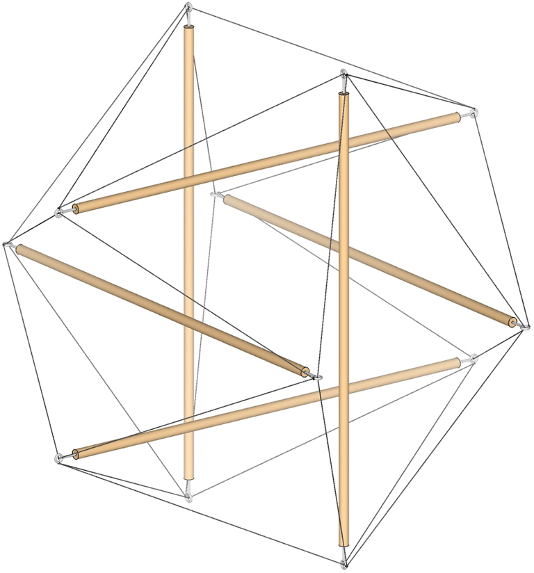
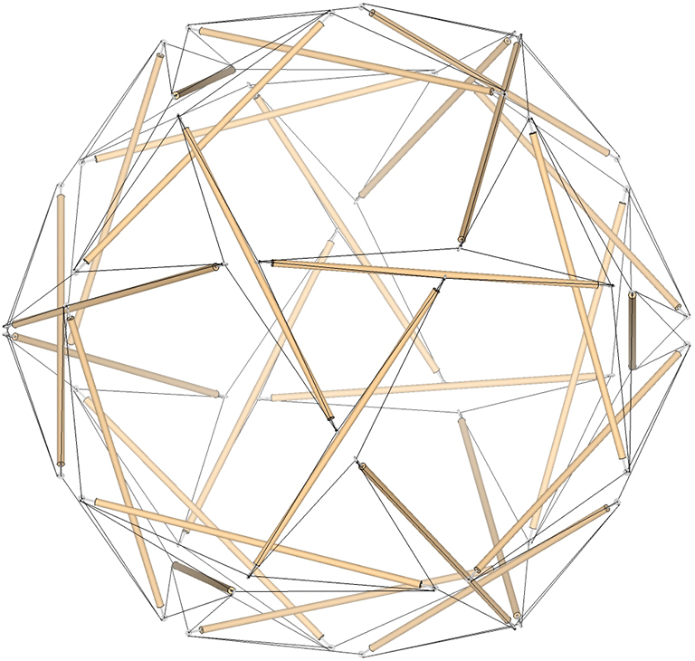
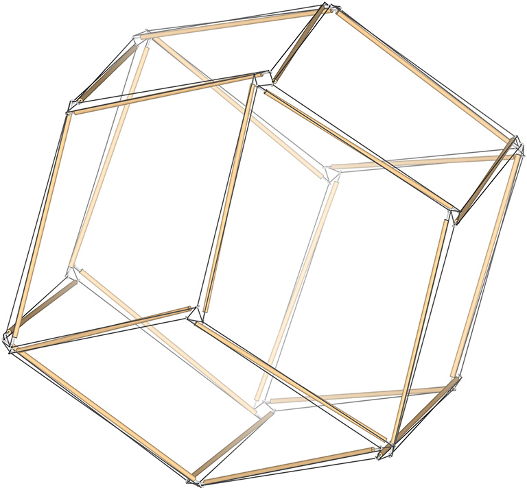
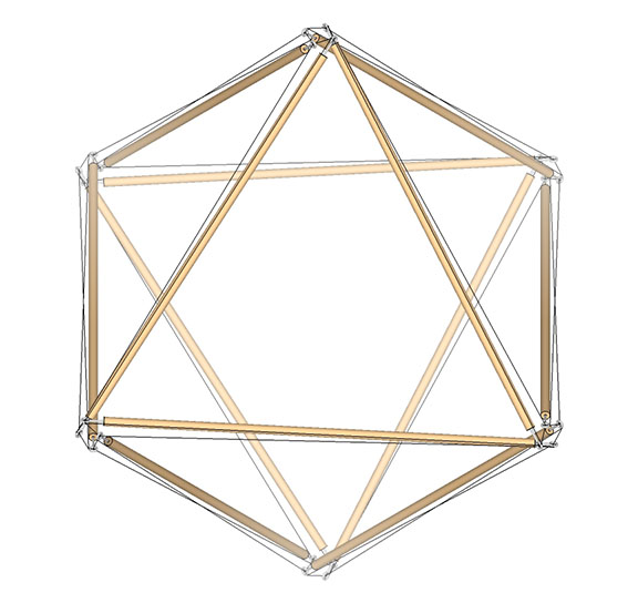
The 6-strut tensegrity sphere is the spherical, or tensor equilibrium phase of the tensegrity tetrahedron and its dual, which is the same tensegrity tetrahedron but with a 90° rotation and with vertices oriented counter-clockwise to the other.
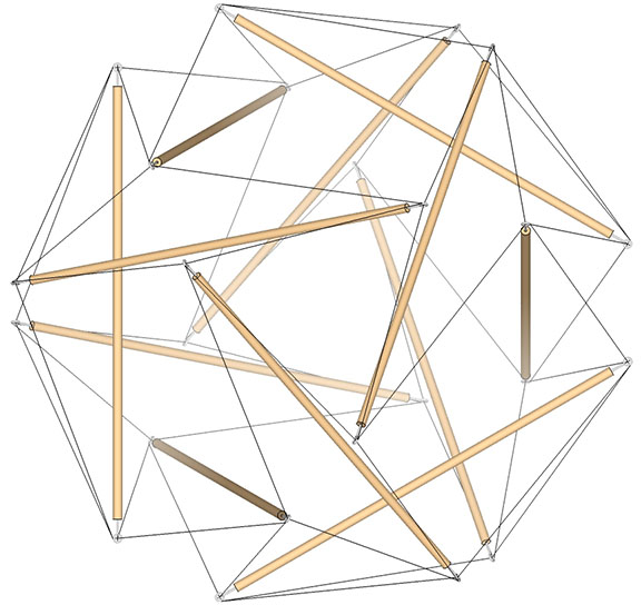
The 6-strut tensegrity sphere.
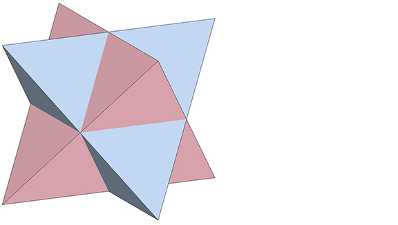
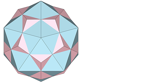
The dual of the regular tetrahedron is conventionally described as the same tetrahedron. Its dual is here described as the negative of the other.
The positive tetrahedron (blue) and its dual, the negative tetrahedron (pink). Note that the vertices in one are the faces in the other, and vice versa.
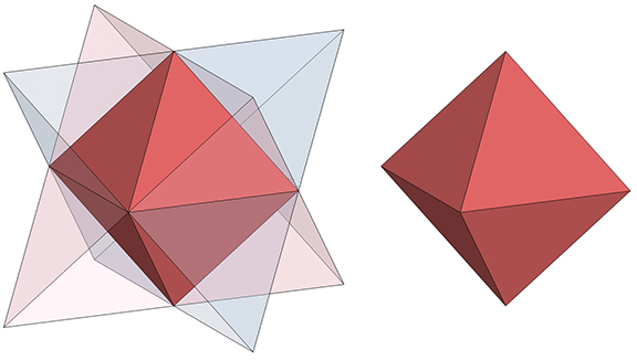
Rectification of either (or the intersection of both) produces the regular octahedron.
Rectification of either (or the intersection of both) a positive and negative tetrahedron (left) produces the octahedron. Note that the edges of the two tetrahedra cross at the vertices of the octahedron.
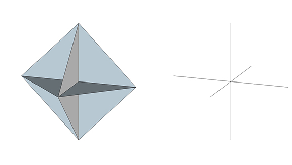
The 12 edges of the octahedron describe three intersecting squares. Connecting alternate vertices of these squares describes three intersecting lines aligned with the distribution of the struts in the 6-strut tensegrity sphere. For consistency, the three lines are here described as three 2-sided polygons, all sharing a common center and each intersecting the other at 90°.
The 12 edges of the octahedron describe three intersecting squares (left). Connecting alternate vertices describes three intersecting lines, or what we’re calling 2-sided polygons (right).
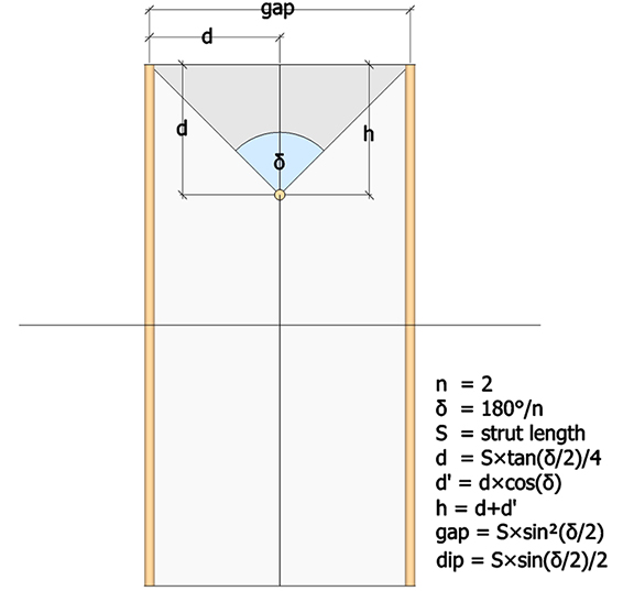
Each of the three intersecting lines (or 2-sided polygons) of the 6-strut tensegrity sphere consists of two struts and the triangular cross section of the valley formed by the tendons connecting each strut-pair to its dangler. The dimensions of this triangular cross-section are illustrated below.
n (number of sides of the polygon) = 2
δ (interior angle of the polygon) = 90°
S = strut length
d (vertical distance from polygon’s edge to strut) = S×tan(δ/2)/4
d’ (height of the triangle formed by the strut ends and the polygon’s vertex) = d×cos(δ) = 0
h (height of the triangle formed by the strut ends and the midpoint of their dangler strut) = (d+d’) = (d+0) = d.
gap (distance between strut ends) = S×sin²(δ/2)/2
dip (distance from strut end to midpoint of dangler strut) = S×sin(δ/2)/2
Dimensions of the cross section of the tension valley formed by the four tendons of a strut pair and their dangler in the 6-strut tensegrity sphere.
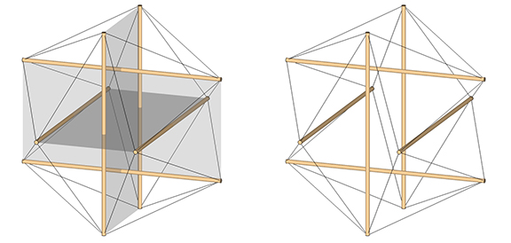
In its spherical, or equilibrium phase, the dimensions of the cross section of the tension valley created by the tendons reach their maximum. In the polyhedral phases described below, δ approaches to 0°, and both the gap and dip go to zero (0).
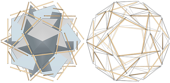
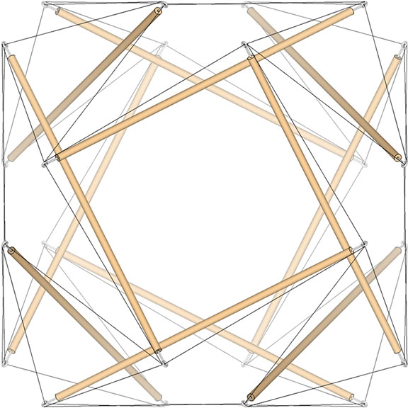
In its spherical, or equilibrium phase, the struts are at their maximum distance from the unit edges of the three intersecting 2-sided polygons (left) of the 6-strut tensegrity sphere (right). For clarity, the 2-sided polygons are shown as transparent rectangles.
Transformation of the 6-Strut Tensegrity Sphere into Positive (or Clockwise) and Negative (or Counter-Clockwise) Tetrahedron.
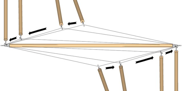
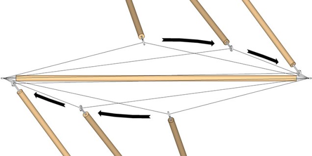
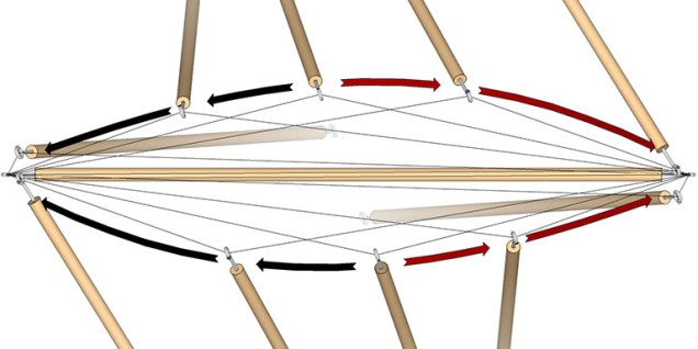
From the spherical phase, the 6-strut tensegrity sphere is reduced to the tensegrity tetrahedron by sliding the strut ends along the tendon toward opposing ends of their dangler, as illustrated below.
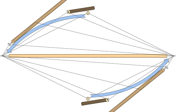
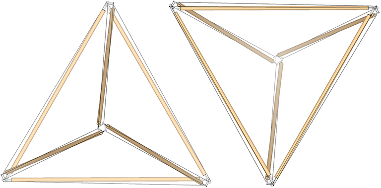
Moving the struts in one direction results in the positive tensegrity tetrahedron…
In the transformation from 6-strut tensegrity sphere to tensegrity tetrahedron, the strut ends move along the tendon to opposing ends of their dangler.
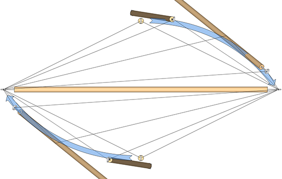
…and moving the struts in the opposite direction results in the negative tensegrity tetrahedron.
In the transformation to the negative tensegrity tetrahedron, the strut ends swap positions at opposing ends of their dangler
The surface of the 6-strut tensegrity sphere describes eight triangular tendon-loops. In the transition to the tetrahedron, four transform into the tetrahedron’s four faces, and the other four transform into the tetrahedrons four vertices. Their roles are swapped in the transformation to the negative tetrahedron.
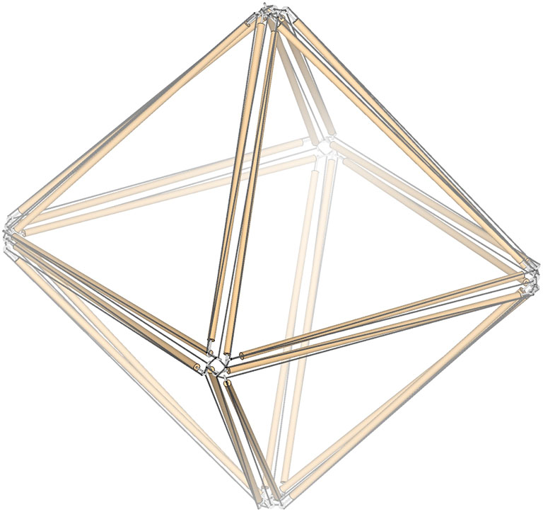
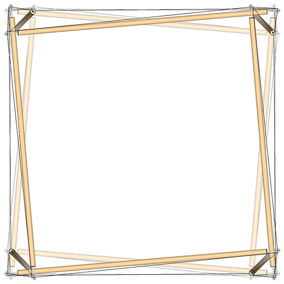
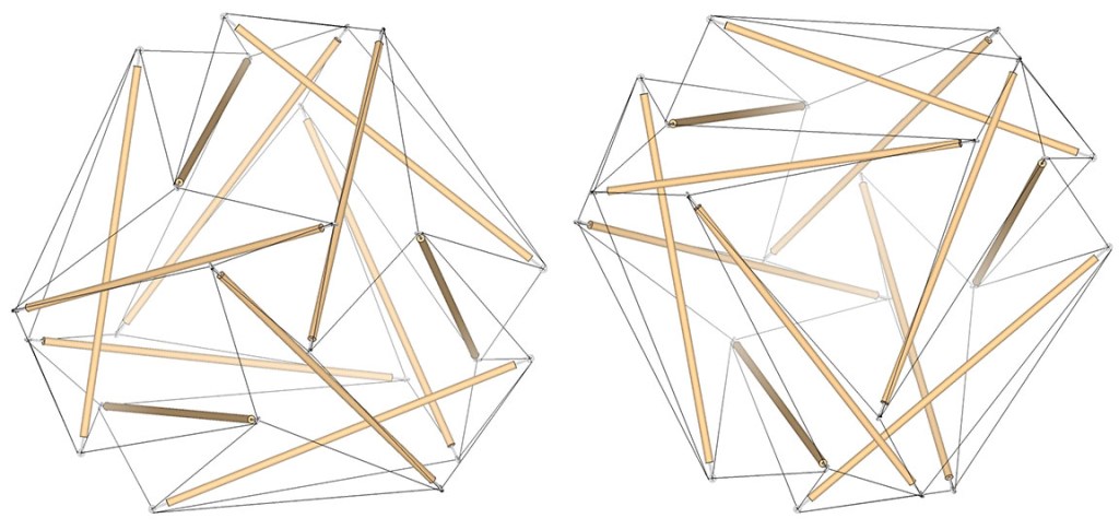
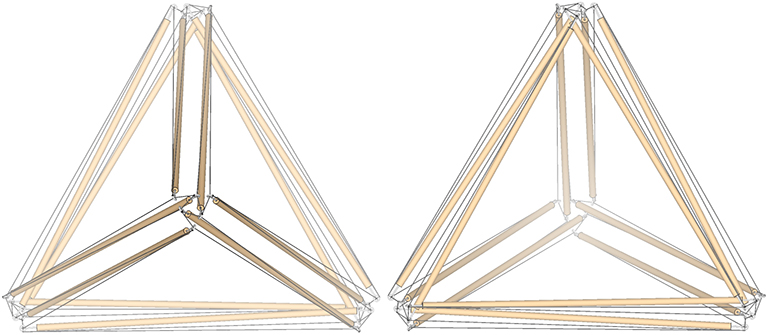
The oscillation of the 6-strut tensegrity sphere produces both the clockwise (or positive) tensegrity tetrahedron (right), and the counter-clockwise (or negative) tetrahedron (left).
The oscillation from the tensor equilibrium (spherical) phase, to the extremes of the two tetrahedron phases, may be stopped at any point and the model will hold its shape. As long as the elasticity and tautness of the tendons is maintained, the models do not show a preference for one state over another.
6-strut tensegrity sphere oscillates smoothly from its spherical phase, between the extreme of its polyhedron phases (the positive and negative tensegrity tetrahedron) all the time holding its shape and showing no preference for one phase over another. .
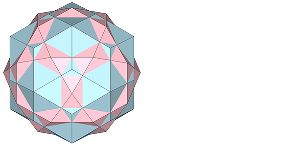
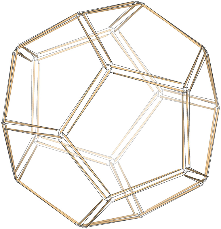
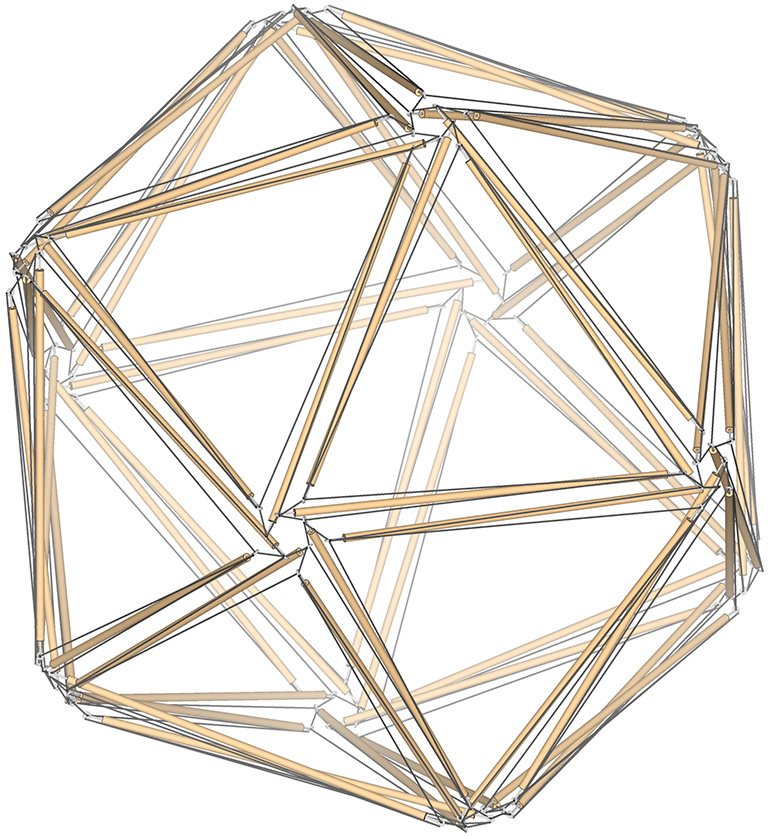
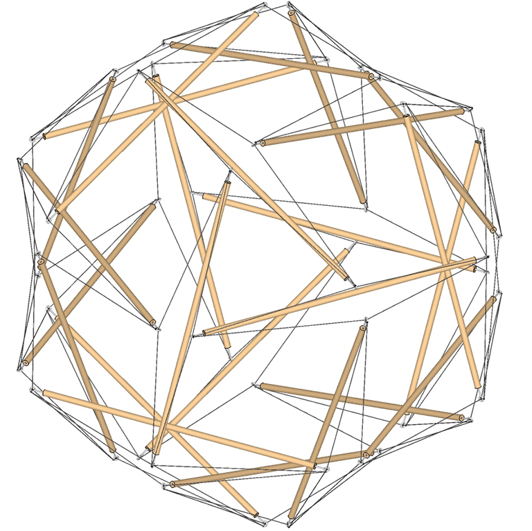
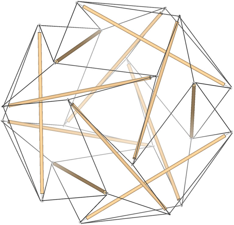
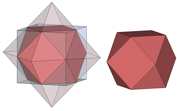
The 30-strut tensegrity sphere is the spherical, or tensor equilibrium phase of the regular icosahedron and its dual, the pentagonal dodecahedron.
30-Strut Tensegrity Sphere
The pentagonal dodecahedron is the dual of the icosahedron.
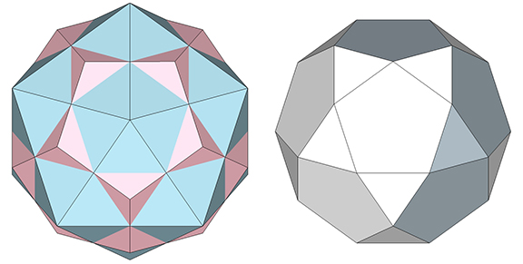
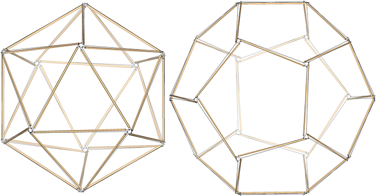
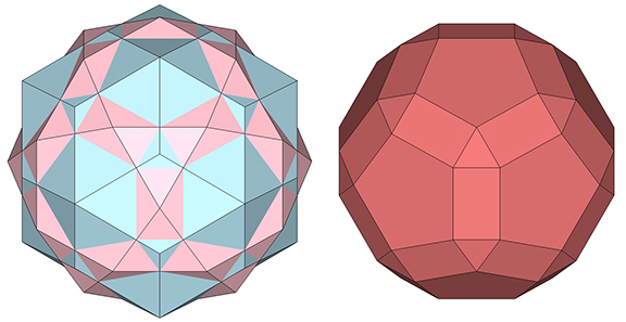
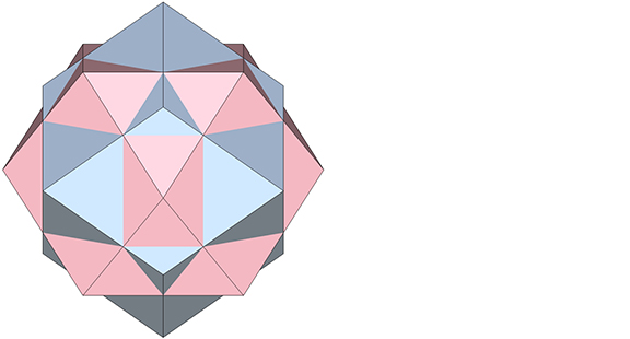
The regular icosahedron (blue) and its dual, the pentagonal dodecahedron (pink). Note that the vertices in one are the faces in the other, and vice versa.
Rectification of either (or the intersection of both) produces the icosidodecahedron.
Rectification of either the regular icosahedron or pentagonal dodecahedron (left), or the intersection of both, produces the icosidodecahedron (right). Note that the edges of the regular icosahedron and the pentagonal dodecahedron cross at the vertices of the icosidodecahedron.
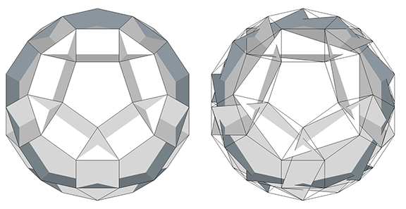
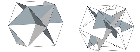
The 60 edges of a icosidodecahedron consist of six intersecting decagons (10-sided polygons). Connecting alternate vertices of the six decagons produces six pentagons whose edges align with the distribution of the struts in the 30-strut tensegrity sphere.
The 60 edges of the icosidodecahedron describe six intersecting decagons (left). Connecting alternate vertices describes six intersecting pentagons (right) whose edges align with the distribution of struts in the 30-strut tensegrity sphere.
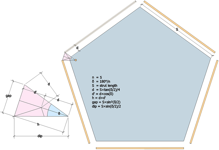
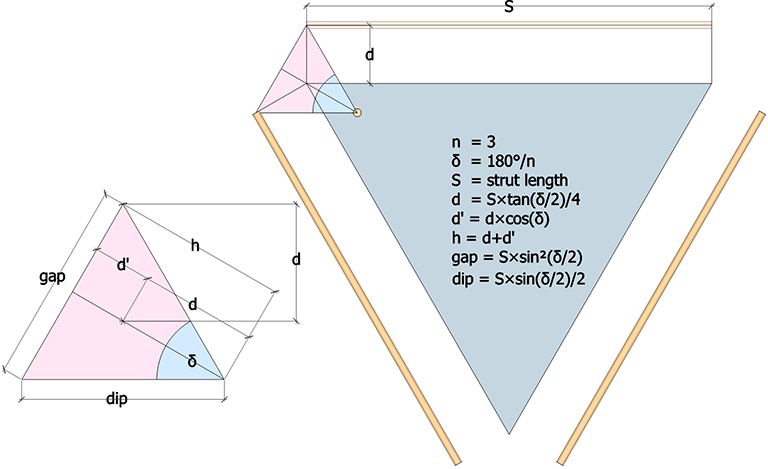
Each of the six intersecting pentagons of the 30-strut tensegrity sphere consists of five struts and the triangular cross section of the valley formed by the tendons connecting each strut-pair to its dangler. The dimensions of this triangular cross-section are illustrated below.
n (number of sides of the polygon) = 5
δ (interior angle of the polygon) = 36°
S = strut length
d (vertical distance from polygon’s edge to strut) = S×tan(δ/2)/4
d’ (height of the triangle formed by the strut ends and the polygon’s vertex) = d×cos(δ)
h (height of the triangle formed by the strut ends and the midpoint of their dangler strut) = d+d’
gap (distance between strut ends) = S×sin²(δ/2)/2
dip (distance from strut end to midpoint of dangler strut) = S×sin(δ/2)/2
Dimensions of the cross section of the tension valley formed by the four tendons of a strut pair and their dangler in the 30-strut tensegrity sphere.
In its spherical, or equilibrium phase, the dimensions of the cross section of the tension valley created by the tendons reach their maximum. In its polyhedral phases (described below), δ approaches 0°, and both the gap and dip approach zero (0).
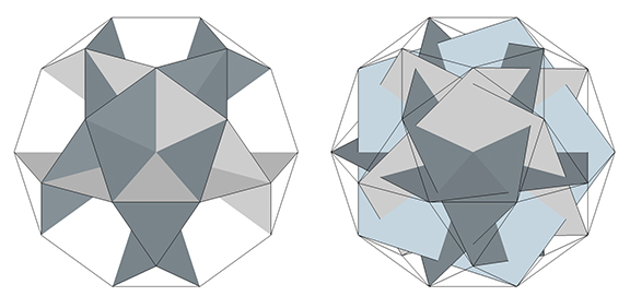
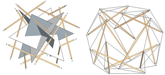
In its spherical, or equilibrium phase, the struts are at their maximum distance from the unit edges of the six intersecting pentagons (left) of the 30-strut tensegrity sphere (right)
Transformation of the 30-Strut Tensegrity Sphere to the Tensegrity Icosahedron and the Tensegrity Pentagonal Dodecahedron
From the spherical phase, the 30-strut tensegrity sphere is reduced to the tensegrity icosahedron by moving each strut along the short tendon toward the end of its dangler, as illustrated below.
In the transformation from 30-strut tensegrity sphere to tensegrity icosahedron, each strut end moves along the short tendon to the end of its dangler.
The sphere is reduced to the tensegrity pentagonal dodecahedron by moving each strut along the long tendon toward the end of its dangler, as illustrated below.
In the transformation from 30-strut tensegrity sphere to tensegrity pentagonal dodecahedron, each strut end moves along the long tendon to the end of its dangler.
The surface of the 30-strut tensegrity sphere describes twenty triangular tendon-loops, and twelve pentagonal tendon-loops. In the transition to the icosahedron, the twenty triangular tendon loops transform into the icosahedron’s twenty faces, and the twelve pentagonal loops transform into its twelve vertices. In the transition to the pentagonal dodecahedron, the roles are reversed: the twenty triangular loops become its vertices, and the twelve pentagonal loops become its faces.
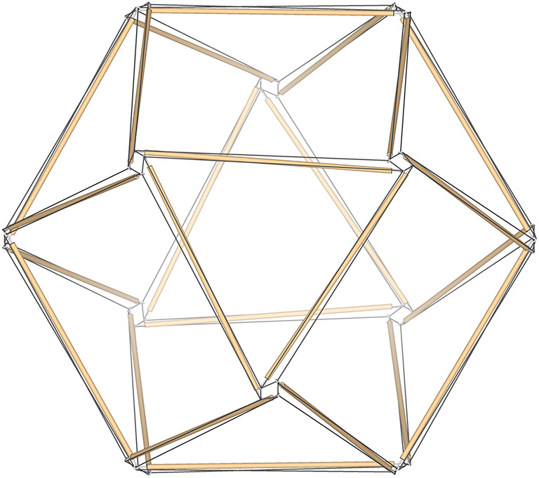
30-strut tensegrity icosahedron (left) and 30-strut tensegrity pentagonal dodecahedron (right)
The oscillation from the tensor equilibrium (spherical) phase, to the extremes of the icosahedron and pentagonal dodecahedron phases, may be stopped at any point and the model will hold its shape. As long as the elasticity and tautness of the tendons is maintained, the models do not show a preference for one state over another.
The 30-strut tensegrity oscillates smoothly from its spherical phase, between the extremes of its polyhedron phases, all the time holding its shape and showing no preference for one phase over another.
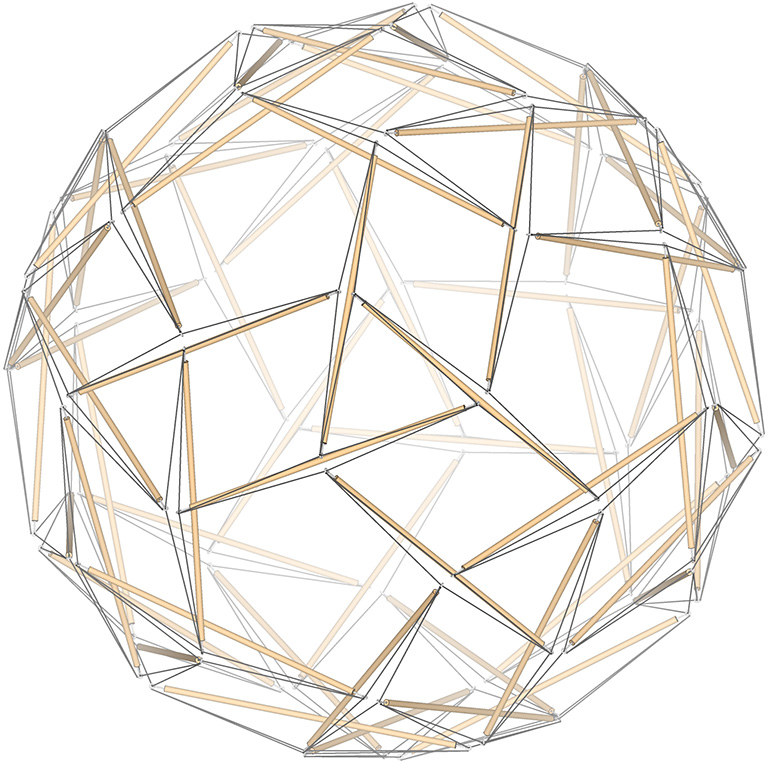
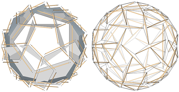
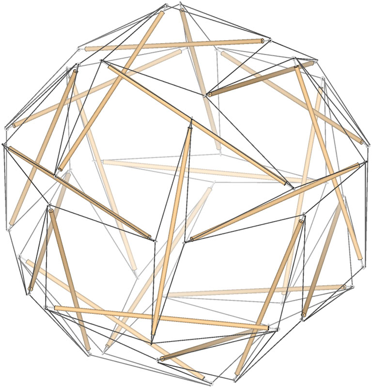
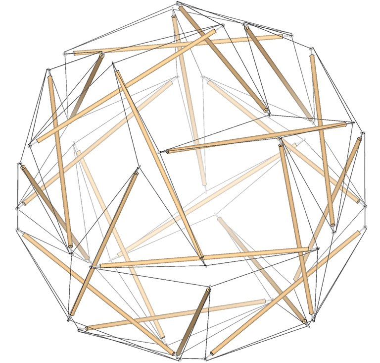
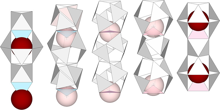
The 60-strut tensegrity sphere is the spherical, or tensor equilibrium phase of the rhombic triacontahedron and its dual, the icosidodecahedron. It also reduces to the double-edge icosahedron and its dual, the double-edge pentagonal dodecahedron.
The 60-strut tensegrity sphere
The rhombic triacontahedron is the dual of the icosidodecahedron.
The rhombic triacontahedron (blue) and its dual, the icosidodecahedron (pink). Note that the vertices in one are the faces in the other, and vice versa.
Rectification of either (or the intersection of both) produces a non-uniform rhombicosidodecahedron.
Rectification of either the rhombic triacontahedron or the icosidodecahedron (left), or the intersection of both, produces the rhombicosadodecahedron (right). Note that the edges of the rhombic triacontahedron and icosidodecahedron cross at the vertices of the rhombicosidodecahedron.
The 120 edges of a rhombicosadodecahedron consist of twelve intersecting decagons (10-sided polygons). If we make the twelve decagons uniform and connect alternate vertices, we produce twelve pentagons whose edges align with the distribution of the struts in the 60-strut tensegrity sphere.
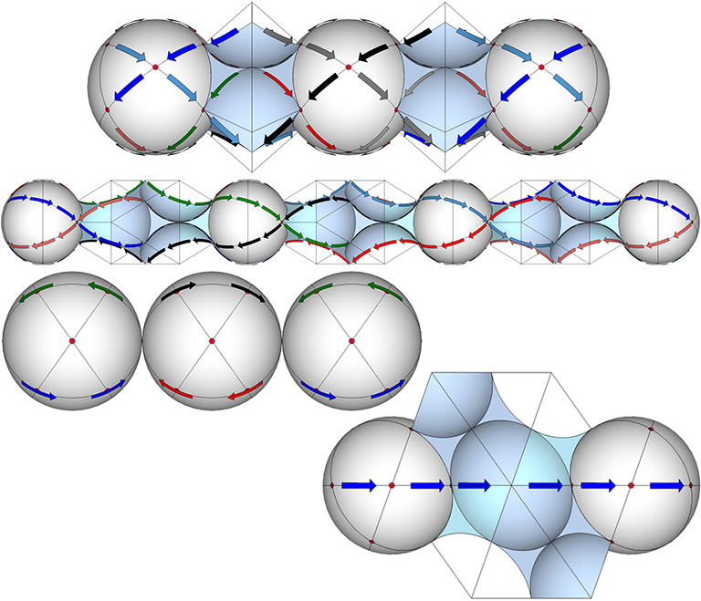
The 120 edges of the uniform rhombicosidodecahedron describe twelve intersecting decagons (left). Connecting alternate vertices describes twelve intersecting pentagons (right) whose edges align with the distribution of struts in the 60-strut tensegrity sphere.
Each of the twelve intersecting pentagons of the 60-strut tensegrity sphere consists of five struts and the triangular cross section of the valley formed by the tendons connecting each strut-pair to its dangler. The dimensions of this triangular cross-section are illustrated below.
n (number of sides of the polygon) = 5
δ (interior angle of the polygon) = 36°
S = strut length
d (vertical distance from polygon’s edge to strut) = S×tan(δ/2)/4
d’ (height of the triangle formed by the strut ends and the polygon’s vertex) = d×cos(δ)
h (height of the triangle formed by the strut ends and the midpoint of their dangler strut) = d+d’
gap (distance between strut ends) = S×sin²(δ/2)/2
dip (distance from strut end to midpoint of dangler strut) = S×sin(δ/2)/2
Dimensions of the cross section of the tension valley formed by the four tendons of a strut pair and their dangler in the 60-strut tensegrity sphere.
In its spherical, or equilibrium phase, the dimensions of the cross section of the tension valley created by the tendons reach their maximum. In its polyhedral phases (described below), δ approaches to 0°, and both the gap and dip go to zero (0).
In its spherical, or equilibrium phase, the struts are at their maximum distance from the unit edges of the twelve intersecting pentagons (left) of the 60-strut tensegrity sphere (right)
Transformation of the 60-Strut Tensegrity Sphere to the Tensegrity Rhombic Triacontahedron
From the spherical phase, the 60-strut tensegrity sphere is reduced to the tensegrity rhombic triacontahedron by moving each strut along the short tendon toward the end of its dangler, as illustrated below.
In the transformation from the 60-strut tensegrity sphere to the tensegrity rhombic triacontahedron, each strut moves along the short tendon to the end of its dangler
The surface of the 60-strut tensegrity sphere describes twenty triangular tendon-loops, twelve pentagonal tendon-loops, and thirty rhombic loops.
In the transition to the rhombic triacontahedron, the thirty rhombic tendon loops transform into the rhombic triacontahedron’s thirty rhombic faces, the twelve pentagonal loops and twenty triangular loops transform into its 5- and 3-vector vertices respectively.
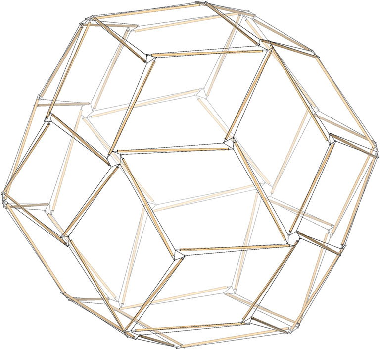
Tensegrity Rhombic Triacontahedron
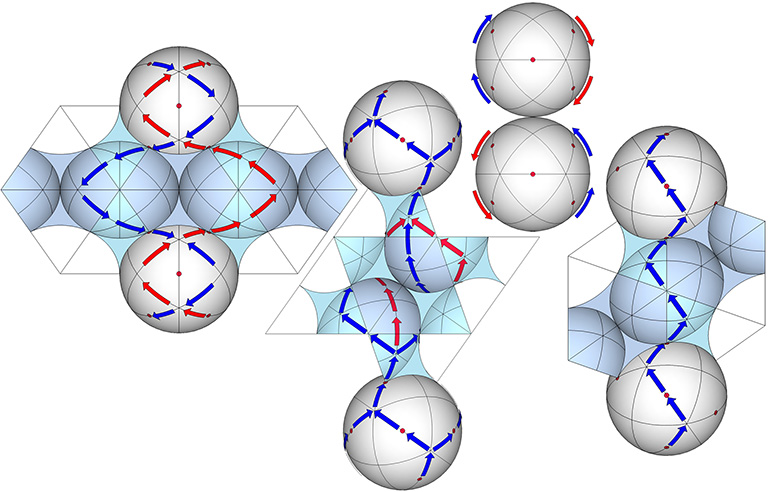
60-strut tensegrity transforming from its spherical phase to the rhombic triacontahedron.
Transformation of the 60-Strut Tensegrity Sphere to the Tensegrity Icosidodecahedron
From its spherical phase, the 60-strut tensegrity sphere is reduced to the tensegrity icosidodecahedron by moving each strut along the long tendon toward the end of its dangler, as illustrated below.
In the transformation from 60-strut tensegrity sphere to the tensegrity icosidodecahedron, each strut end moves along the long tendon to the end of its dangler.
In the transition to the icosidodecahedron, the thirty rhombic tendon loops transform into the icosidodecahedron’s thirty vertices, while the the twelve pentagonal and twenty triangular loops transform into its twelve pentagonal and twenty triangular faces.
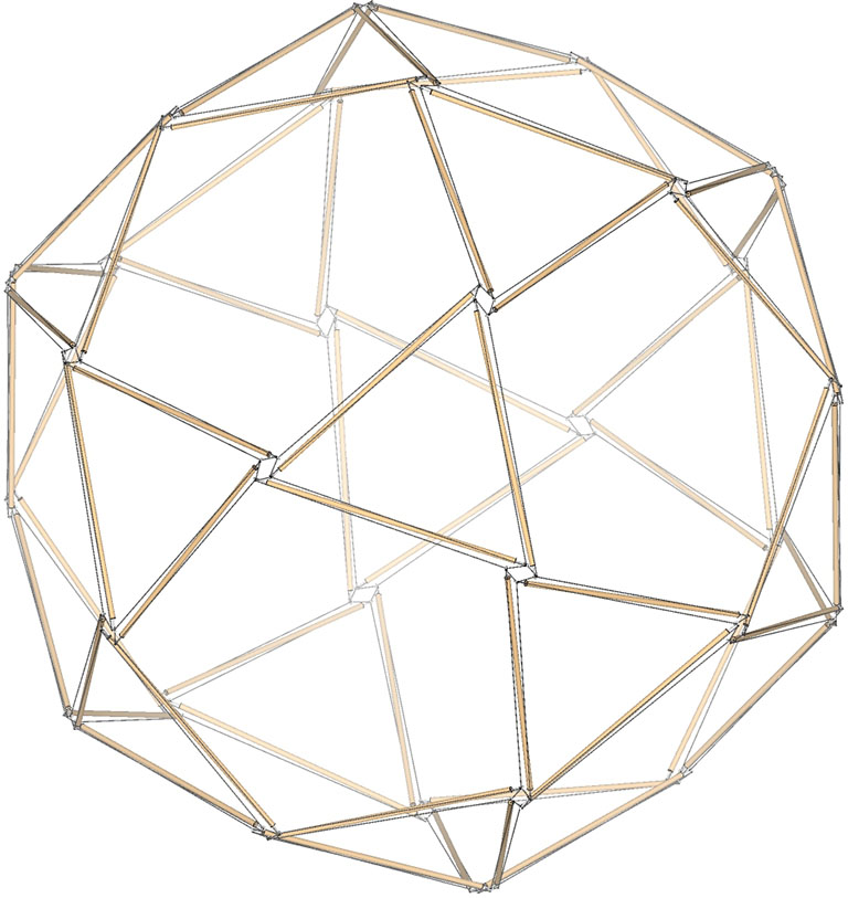
60-strut tensegrity icosidodecahedron
60-strut tensegrity transforming from its spherical phase to the icosidodecahedron.
Transformation of the 60-Strut Tensegrity Sphere to Double-Edge Tensegrity Pentagonal Dodecahedron
From its spherical phase, the 60-strut tensegrity can be transformed into a double-edge pentagonal dodecahedron or a double-edge icosahedron by moving the strut pairs together to either the left or right end of their danglers. That is, one strut moves along the short tendon, while the other moves along the long tendon toward the same end of their dangler.
In the transformation from 60-strut tensegrity sphere to the double-edge tensegrity pentagonal dodecahedron, each strut pair moves in the same direction to one end or the other of their dangler.
In the illustration below, the 60-strut tensegrity sphere’s twenty triangular loops have contracted to form the vertices of the double-edge pentagonal dodecahedron, while the twelve pentagonal tendon loops have expanded into its twelve pentagonal faces, and the thirty rhombic tendon loops have transformed into its thirty edges.
60-strut tensegrity transforming between its spherical phase and the double-edge pentagonal dodecahedron.
Transformation of the 60-Strut Tensegrity Sphere to the Double-Edge Tensegrity Icosahedron
In the illustration below, the twelve pentagonal loops have contracted to form the twelve vertices of the double-edge tensegrity icosahedron, while the twenty triangular tendon loops have expanded into its twenty faces, and the thirty rhombic tendon loops have transformed into its thirty edges.
60-strut double-edge tensegrity icosahedron.
60-strut tensegrity transforming between its spherical phase and the double-edge tensegrity icosahedron.
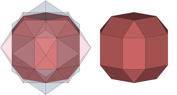
The 24-strut tensegrity sphere is the spherical, or tensor equilibrium phase of the tensegrity rhombic dodecahedron and its dual, the tensegrity vector equilibrium (VE). It also reduces to the double-edge tensegrity octahedron and its dual, the double-edge tensegrity cube.
The 24-strut tensegrity sphere.
The rhombic dodecahedron is the dual of the vector equilibrium (VE).
The rhombic dodecahedron (blue) and its dual, the vector equilibrium or VE (pink). Note that the vertices in one are the faces in the other, and vice versa.
Rectification of either (i.e., the intersection of both) produces a non-uniform rhombicuboctahedron.
Rectification of either the rhombic dodecahedron or the vector equilibrium (left) produces the rhombicuboctahedron (right). Note that the edges of the rhombic dodecahedron and vector equilibrium cross at the vertices of the rhombicuboctahedron.
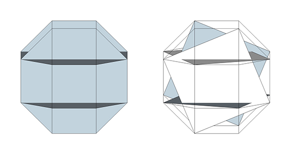
The 48 edges of a rhombicuboctahedron consist of six intersecting octagons. If we make the six octagons uniform and connect alternate vertices, we produce six squares whose edges align with the distribution of the struts in the 24-strut tensegrity sphere.
The 48 edges of the uniform rhombicuboctahedron describe six intersecting octagons (left). Connecting alternate vertices describes six intersecting squares (right).
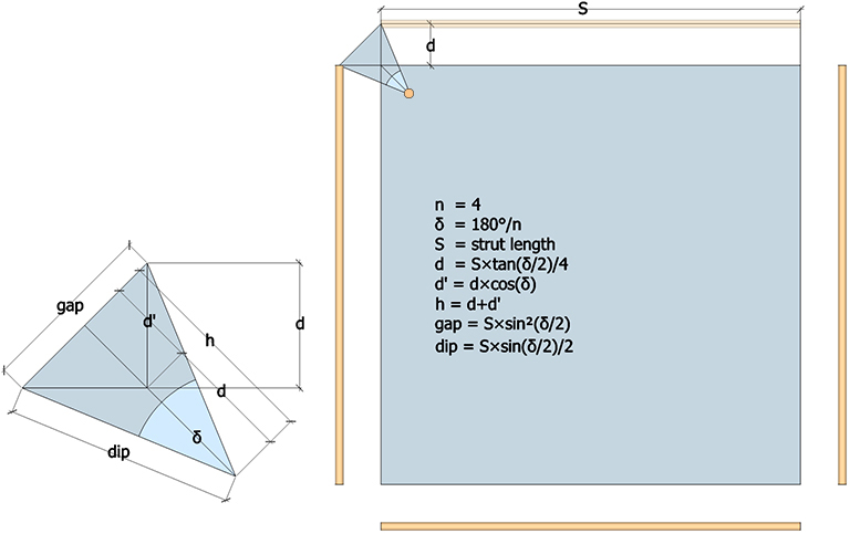
Each of the six intersecting squares of the 24-strut tensegrity sphere consists of four struts and the triangular cross section of the valley formed by the tendons connecting each strut-pair to its dangler. The dimensions of this triangular cross-section are illustrated below.
n (number of sides of the polygon) = 4
δ (interior angle of the polygon) = 45°
S = strut length
d (vertical distance from polygon’s edge to strut) = S×tan(δ/2)/4
d’ (height of the triangle formed by the strut ends and the polygon’s vertex) = d×cos(δ)
h (height of the triangle formed by the strut ends and the midpoint of their dangler strut) = d+d’
gap (distance between strut ends) = S×sin²(δ/2)/2
dip (distance from strut end to midpoint of dangler strut) = S×sin(δ/2)/2
Dimensions of the cross section of the tension valley formed by the four tendons of a strut pair and their dangler in the 24-strut tensegrity sphere.
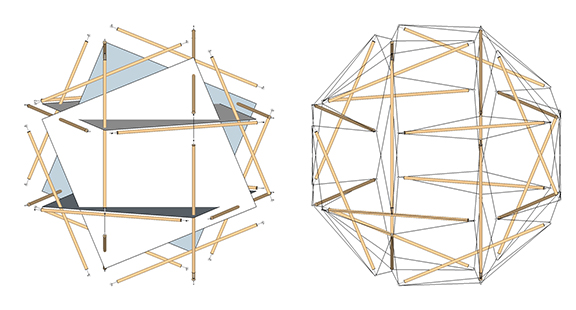
In its spherical, or equilibrium phase, the dimensions of the cross section of the tension valley created by the tendons reach their maximum. In the polyhedral phases described below, δ approaches to 0°, and both the gap and dip go to zero (0).
In its spherical, or equilibrium phase, the struts are at their maximum distance from the unit edges of the six intersecting squares (left) of the 24-strut tensegrity sphere (right).
Transformation of the 24-Strut Tensegrity Sphere to the Tensegrity Vector Equilibrium (VE)
From the spherical phase, the 24-strut tensegrity sphere is reduced to the tensegrity VE by moving each strut along the long tendon toward the end of its dangler, as illustrated below.
In the transformation from 24-strut tensegrity sphere to the tensegrity VE, each strut end moves along its long tendon to the end of its dangler.
The surface of the 24-strut tensegrity sphere describes eight triangular tendon-loops, six square tendon-loops, and twelve rhombic loops. A face-on view of one of the triangular tendon loops is illustrated below.
24-strut tensegrity in its spherical phase with the view oriented on one of its eight equilateral triangle tendon loops.
In the transition to the VE, the eight triangular tendon loops transform into the VE’s eight triangular faces, the six square tendon loops transform into the VE’s six square faces, and the twelve rhombic loops transform into the VE’s twelve vertices.
24-strut tensegrity vector equilibrium (VE)
24-strut tensegrity transforming between its spherical phase and the tensegrity VE.
Transformation of the 24-Strut Tensegrity Sphere to the Tensegrity Rhombic Dodecahedron
From the spherical phase, the 24-strut tensegrity sphere is reduced to the tensegrity rhombic dodecahedron by moving each strut along the short tendon toward the end of its dangler, as illustrated below.
In the transformation from the 24-strut tensegrity sphere to the tensegrity rhombic dodecahedron, each strut moves along the short tendon to the end of its dangler
The surface of the 24-strut tensegrity sphere describes eight triangular tendon-loops, six square tendon-loops, and twelve rhombic loops. One of the twelve rhombic tendon loops is right-center in the illustration below.
24-strut tensegrity sphere viewed with one of its twelve rhombic tendon loops face-on right of center.
In the transition to the rhombic dodecahedron, the twelve rhombic tendon loops transform into the rhombic dodecahedron’s twelve rhombic faces, the six square tendon loops transform into its six 4-strut vertices, and the eight triangular loops transform into its eight 3-strut vertices.
24-strut rhombic dodecahedron
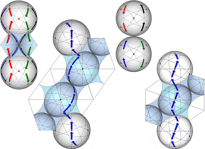
24-strut tensegrity transforming between its spherical phase and the tensegrity rhombic dodecahedron.
Transformation of the 24-Strut Tensegrity Sphere to the Double-Edged Tensegrity Octahedron
From its spherical phase, the 24-strut tensegrity can be transformed into a double-edge octahedron or a double-edge VE by moving the strut pairs together to either the left or right end of their danglers. That is, one strut moves along the short tendon, while the other moves along the long tendon toward the same end of their dangler.
In the transformation from 24-strut tensegrity sphere to the double-edge tensegrity octahedron or VE, each strut pair moves in the same direction to one end or the other of their dangler.
The surface of the 24-strut tensegrity sphere describes eight triangular tendon-loops, six square tendon-loops, and twelve rhombic tendon-loops. In the illustration below, the six square loops have contracted to the vertices of the double-edge octahedron, while the eight triangular tendon loops have expanded into its eight faces, and the twelve rhombic tendon loops have transformed into its twelve edges.
24-strut double-edge octahedron
24-strut tensegrity transforming between its spherical phase and the double-edge tensegrity octahedron.
Transformation of the 24-Strut Tensegrity Sphere to the Double-Edged Tensegrity Cube
The surface of the 24-strut tensegrity sphere describes eight triangular tendon-loops, six square tendon-loops, and twelve rhombic tendon-loops. In the illustration below, the eight triangular loops have contracted to the vertices of the double-edge cube, while the six square tendon loops have expanded into its eight faces, and the twelve rhombic tendon loops have transformed into its twelve edges.
24-strut double-edge tensegrity cube.
24-strut tensegrity transforming between its spherical phase and the double-edge tensegrity cube.
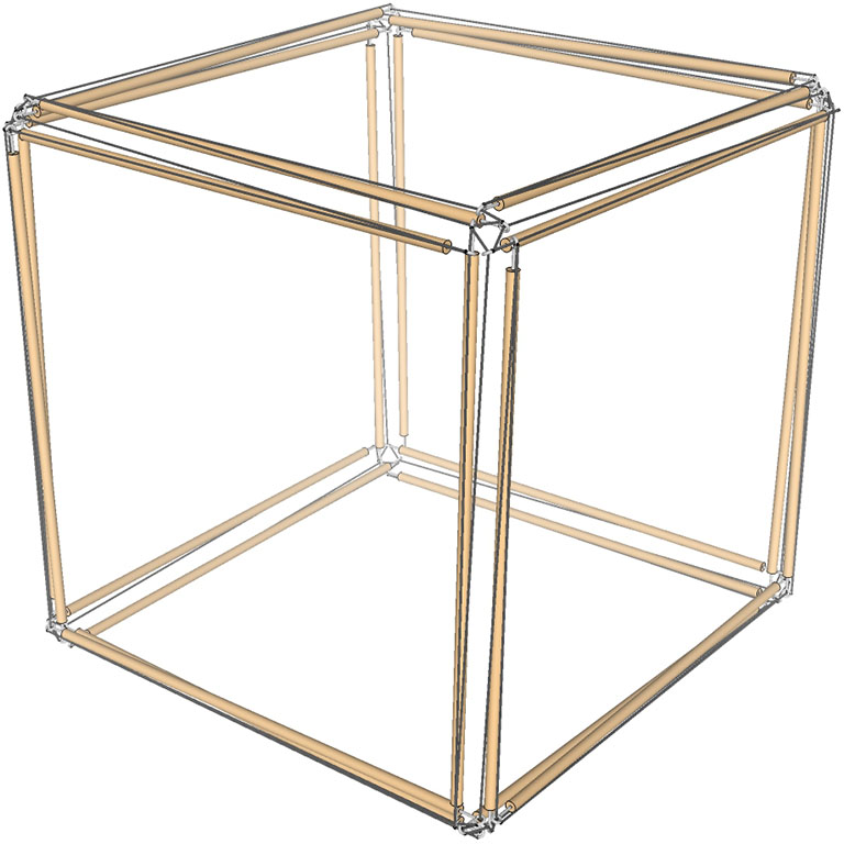
The 12-strut tensegrity sphere is the spherical, or tensor equilibrium phase of the tensegrity cube and its dual, the tensegrity octahedron. It also reduces to the double-edge tensegrity tetrahedron and its dual, which is the same polyhedron but with the vertices and faces transposed.
12-strut tensegrity sphere.
The cube is the dual the regular octahedron.
The cube (blue) and its dual, the regular octahedron (pink). Note that the vertices in one are the faces in the other, and vice versa.
Rectification of either produces the cuboctahedron, i.e, the vector equilibrium or VE.
Rectification of either (or the intersection of both) the cube or the regular octahedron (left) produces the cuboctahedron, i.e. vector equilibrium or VE (right). Note that the edges of the cube and regular octahedron cross at the vertices of the VE.
The 24 edges of the VE describe four intersecting hexagons. Connecting alternate vertices of these hexagons describes four equilateral triangles whose edges align with the distribution of the struts in the 12-strut tensegrity sphere.
The 24 edges of the VE describe four intersecting hexagons (left). Connecting alternate vertices describes four intersecting equilateral triangles (right).
Each of the four intersecting triangles of the 12-strut tensegrity sphere consists of three struts and the triangular cross section of the valley formed by the tendons connecting each strut-pair to its dangler. The dimensions of this triangular cross-section are illustrated below.
n (number of sides of the polygon) = 3
δ (interior angle of the polygon) = 60°
S = strut length
d (vertical distance from polygon’s edge to strut) = S×tan(δ/2)/4
d’ (height of the triangle formed by the strut ends and the polygon’s vertex) = d×cos(δ)
h (height of the triangle formed by the strut ends and the midpoint of their dangler strut) = d+d’
gap (distance between strut ends) = S×sin²(δ/2)/2
dip (distance from strut end to midpoint of dangler strut) = S×sin(δ/2)/2
Dimensions of the cross section of the tension valley formed by the four tendons of a strut pair and their dangler in the 12-strut tensegrity sphere.
In its spherical, or equilibrium phase, the dimensions of the cross section of the tension valley created by the tendons reach their maximum. In the polyhedral phases described below, δ approaches to 0°, and both the gap and dip go to zero (0).
In its spherical, or equilibrium phase, the struts are at their maximum distance from the unit edges of the four intersecting equilateral triangles (left) of the 12-strut tensegrity sphere (right).
Transformation of the 12-Strut Tensegrity Sphere to the Tensegrity Cube
From the spherical phase, the 12-strut tensegrity sphere is reduced to the tensegrity cube by moving each strut along the short tendon toward the end of its dangler, as illustrated below.
In the transformation from 12-strut tensegrity sphere to tensegrity cube, each strut end moves along the short tendon to the end of its dangler.
The surface of the 12-strut tensegrity sphere describes eight triangular tendon-loops and six square tendon-loops. A face-on view of one of the square tendon loops is illustrated below.
12-strut tensegrity in its spherical phase with the view oriented on one of its six square tendon loops.
In the transition to the cube, the six square tendon loops transform into the cube’s six faces, while the eight triangular loops transform into the cube’s eight vertices.
Tensegrity Cube
12-strut tensegrity transforming between its spherical phase and the tensegrity cube.
Transformation of the 12-Strut Tensegrity Sphere to the Tensegrity Octahedron
From the spherical phase, the 12-strut tensegrity sphere is reduced to the tensegrity octahedron by moving each strut along the long tendon toward the end of its dangler, as illustrated below.
In the transformation from 12-strut tensegrity sphere to the tensegrity octahedron, each strut end moves along its long tendon to the end of its dangler.
The surface of the 12-strut tensegrity sphere describes eight triangular tendon-loops and six square tendon-loops. A face-on view of one of the triangular tendon loops is illustrated below.
The 12-strut tensegrity in its spherical phase oriented on one of its eight triangular tendon loops.
The six square loops of the 12-strut tensegrity sphere reduce to form the six vertices of the tensegrity octahedron, while the eight triangular loops expand of form its eight faces.
Tensegrity Octahedron
The 12-strut tensegrity transforming between its spherical phase and the tensegrity octahedron.
The oscillation from the tensor equilibrium (spherical) phase, to the extremes of the cube and octahedron phases, may be stopped at any point and the model will hold its shape. As long as the elasticity and tautness of the tendons is maintained, the models do not show a preference for one state over another.
12-strut tensegrity oscillates smoothly from its spherical phase, between the extremes of its polyhedron phases, all the time holding its shape and showing no preference for one phase over another.
Note that the orientations (clockwise or counter-clockwise) of the triangular and square loops are mutually opposed. That is, if one is oriented clockwise, then the other will necessarily be counter-clockwise. That is, each polyhedron will always be counter the orientation of its dual at the other extreme of the transformation. This, however, does not seem to be the case for double-edged tetrahedron described below.
Transformation of the 12-Strut Sphere to the Double-Edged Tetrahedron
From its spherical phase, the 12-strut tensegrity can be transformed into a double-edged tetrahedron by moving the strut pairs together to either the left or right end of their danglers. That is, one strut moves along the short tendon, while the other moves along the long tendon toward the same end of their dangler.
In the transformation from 12-strut tensegrity sphere to the double-edge tensegrity tetrahedron, each strut pair moves in the same direction to one end or the other of their dangler.
The surface of the 12-strut tensegrity sphere describes eight triangular tendon-loops and six square tendon-loops. A face-on view of one of the triangular tendon loops is illustrated below. On the left, the triangular loop is contracting to a vertex, while on the right, the triangular loop is expanding to a face. In both cases, the six square tendon loops are transformed into the six edges of the double-edge tetrahedron.
The 12-strut tensegrity approximately midway between its spherical phase and the double-edge tensegrity tetrahedron. Four of the eight triangular tendon loops transform into vertices (left), while the other four transform into faces (right).
Note that both transformations (moving the strut pairs to either end of their danglers) produce the same double-edge tetrahedron. This is consistent with the fact that the tetrahedron is its own dual; the number of faces (4) is the same as the number of vertices (4), so transposing the two has no effect. However, with the other duals, if one’s vertices are oriented clockwise, the other’s are oriented counter-clockwise. With the double-edge tensegrity tetrahedron, the vertices are neither and both: three struts converge at the vertex oriented in one direction, and the other three come together oriented in the opposite direction, one effectively neutralizing the other.
The double-edge tetrahedron and, presumably, all the double-edge tensegrity polyhedra are, by the above reasoning, neutral counterparts to their polarized, single-edge counterparts. This may have intriguing implications for their relevance as models of quantum, chemical, and other physical interactions and open doors for theoretical exploration and research.
The two transformations, moving the strut pairs to one end or the other of their danglers, produces the same double edge tetrahedron.
As with the transformations described above, the oscillations between the two double-edged tetrahedra may be stopped at any point in the process. The models do not some seem to prefer any one state over another, and will hold their shape in the transitional stages as well as at the extremes.
The 12-strut tensegrity transforming between two orientations of the double-edge tetrahedron via its spherical phase.
“Vector equilibrium accommodates all the inter-transformings of any one tetrahedron by polar pumping, or turning itself inside out. Each vector equilibrium has four directions in which it could turn inside out. It uses all four of them through the vector equilibrium’s common center and generates eight tetrahedra. The vector equilibrium is a tetrahedron exploding itself, turning itself inside out in four possible directions. So we get eight: inside and outside in four directions. The vector equilibrium is all eight of the potentials.” —R. Buckminster Fuller, Synergetics, 441.02
The axes of the set of 4 great circles of the vector equilibrium (VE) stands apart from the other three sets in its significance to the rest of Fuller’s geometry:
It is the axis on which the vector model rotates and contracts in the jitterbug transformation. (See: Jitterbug.)
Its four great circles define the spherical vector equilibrium.
The combined area of its four great circle planes is identical with the surface area of the sphere of the same radius.
The axis forms a channel for the polar pump model of the jitterbug transformation, which is the subject of this article.
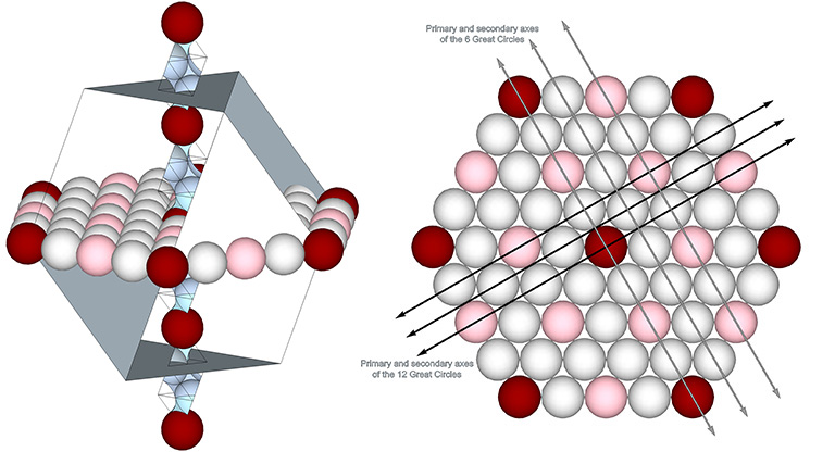
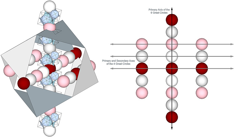
The primary axis of the set of four great circles directly connects each nucleus with 8 of its 14 surrounding nuclei with no intervening spheres between them. Its secondary axes also connect like spheres: nuclear voids with nuclear voids, and; F1 shell spheres with F1 shell spheres. (See: Categories of Spheres in the Isotropic Vector Matrix: Nuclei, F1 Shells, and “Nuclear Voids”). Each sphere is separated along each axis by interstitial space consisting of one concave VE and two concave octahedra. (See: Spaces and Spheres (Redux) and Spheres and Spaces.)
The primary (top) and secondary axes of the 4 Great Circles of the vector equilibrium connect like-with-like spheres, each separated by interstitial space. The jitterbugging matrix may shuttle spheres freely along these axes, leaving its configuration undisturbed.
If we imagine the matrix shuttling spheres exclusively along these axes, each cycle of the jitterbug produces identical results and no change is perceived in the configuration or orientation of the discrete cubes and VEs described in my previous article, Blinkers, the Jitterbug, and the “Crystalized” Isotropic Vector Matrix.
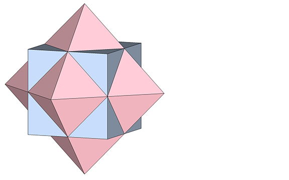
The jitterbug is, essentially, the positive-negative oscillation of tetrahedra, and Fuller consistently viewed this oscillation as the vector equilibrium (VE) exploding itself, its eight tetrahedra forcing their common vertex out through their opposite faces to form the star octahedron, or cube, as illustrated below.
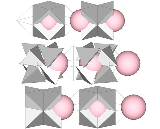
Polar Pump: Each of the eight tetrahedra of the vector equilibrium (upper left) are turned inside out by moving their common vertex at the center of the VE outward while simultaneously jitterbugging to form the star octahedron, or cube (lower right).
The following illustrates how this model of the jitterbug might be conceived as the shuttling of nuclei into and out of the octahedra as they unfold into VEs and fold back again into octahedra. This is the same space-to-sphere, sphere-to-space oscillation as in all other models of the jitterbug—the only difference being the axis along which the adjacent space (the concave VE that is replaced by a sphere) is perceived to lie.
The polar pump restricted to just one of the four axes shows how the inside-outing tetrahedron shuttles the nucleus out of the collapsing VE and into the expanding octahedron.
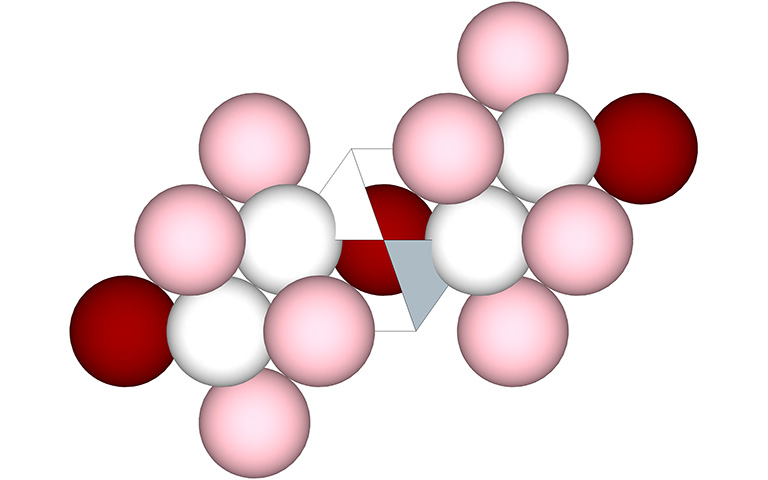
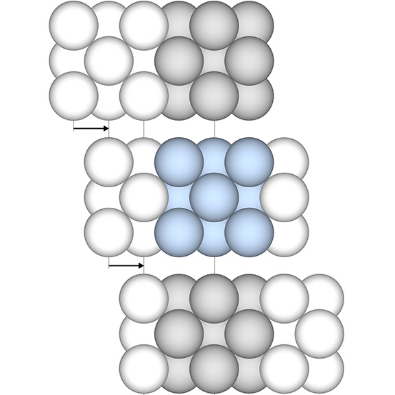
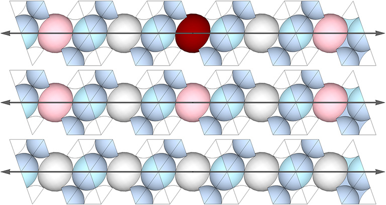
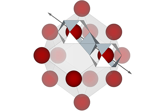
In the illustration below, the six spheres of the octahedron (gray spheres) contribute 3-spheres each to the F1 shells of two nuclei (center) aligned on opposing points of each of the cube’s (right) four diagonals, one of which is the primary axis of the four great circles connecting nuclei (red spheres), and the others are secondary axes connecting nuclear voids (pink spheres). This polarization of the nuclei to just one of the four axes may explain why Fuller referred to its migration along this axis as a “polar” pump.
The star octahedron, or cube (right), sits between VE’s (center) on the primary axis of the four great circles (left). Though four axes pass through the the octahedron/cube, only one connects nuclei (red); the others connect nuclear voids (pink).
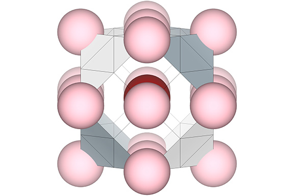
In the following illustration, two of these polarized cubes are shown straddling a VE with which they share a nucleus.
Two octahedra/cubes straddling a nuclear VE (center) on the primary axis of the four great circles.
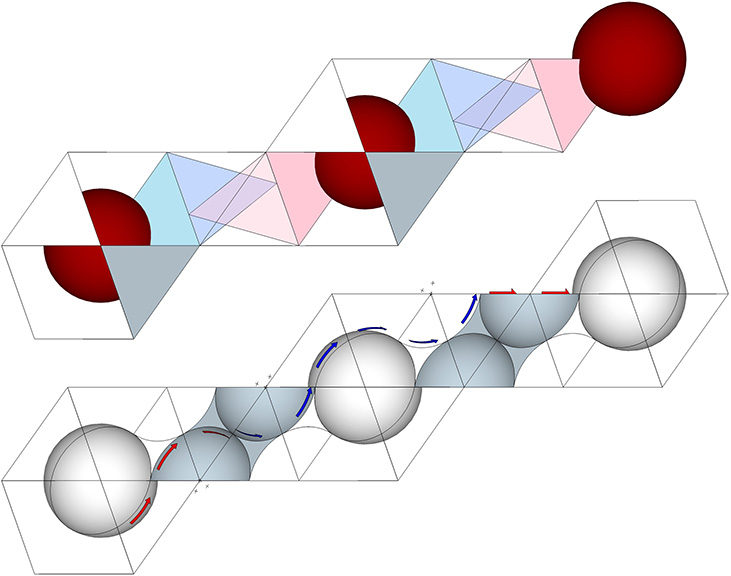
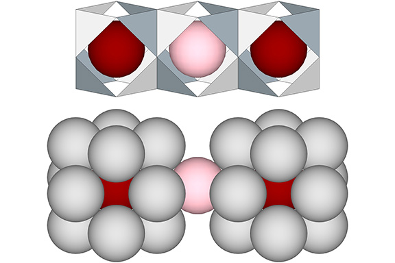
At the top of the illustration below, the cubic clusters of close-packed spheres have been replaced with octahedra, inside of which are the inside-outed tetrahedra from their adjacent VEs. Below that, the octahedra and tetrahedra have been replaced with concave VE spaces and concave octahedron interstices. Arrows indicate how the set of four great circles constitute the shortest-distance geodesics connecting spheres along the axis. Note that the path makes a sharp right angle at the halfway point. For each of the eight possible geodesics (for which only one is shown), the red arrows change to blue arrows at the point of tangency between two of the six spheres of the octahedron that sits between the VEs. This mirrors the positive-negative oscillations of tetrahedra.
The octahedra space through which the axes of the 4 great circles pass accommodates eight inside-outed tetrahedra at the halfway point of the polar pump model of the jitterbug (top). This corresponds to the positive-negative oscillation of tetrahedra in other models of the jitterbug, and is mirrored in the 90° turn of the shortest-distance geodesic path between spheres on the axes (bottom).
Another way of looking that this is to have the tetrahedra unfold and wrap themselves around the octahedra, then unwrap and refold themselves into tetrahedra at the octahedron’s opposite pole.
A positive tetrahedron (left) unfolds and wraps itself around the octahedron space between two VEs (center) before refolding into a negative tetrahedron (right) in this model of the polar pump. Click to view animation under a separate tab.
The octahedron sits between a positive and a negative tetrahedron in the isotropic vector matrix, and accommodates their inside-outing, or positive-negative oscillations, both internally, i.e., as inside-outed tetrahedra clustered inside the octahedron, and externally, i.e., as tetrahedra unfolded and wrapped around its surface. The model provides a way of visualizing the jitterbug transformation on an otherwise fixed matrix.
“We may define the individual as one way the game of Universe could have eventuated to date. Universe is the omnidirectional, omnifrequency game of chess in which with each turn of the play there are 12 vectorial degrees of freedom: six positive and six negative moves to be made. This is a phenomenon of frequencies and periodicities. Each individual is a complete game of Universe from beginning to end.” —R. Buckminster Fuller, Synergetics, 537.41
In previous posts, I’ve suggested that the jitterbug transformation may be associated with the migration of nuclei. The radially close-packed spheres of the isotropic vector matrix divide naturally into clusters in the shape of cubes and vector equilibria (VEs). See Space-Filling Polyhedra as Close-Packed Spheres. In the following illustration I’ve replaced the sphere clusters with tetrahedra. The eight tetrahedra that share a common vertex at the center of the VE are rotated 90°, or “jitterbug”, so that their common vertex faces outward to form the eight points of the cube. If we add the nuclei into this model, it suggests a migration of nuclei between the two.
This model of the jitterbug transformation, in which the eight tetrahedra of the VE are rotated 90° to form the eight points of a cube, suggests the migration of nuclei (pink spheres).
The effect of the jitterbug transformation may also be conceived as the shifting not only of nuclei but of all spheres comprising the isotropic vector matrix into their adjacent spaces. The natural axis for the transformation is that of the 3 Great Circles, the only axis on which every sphere is connected directly through the center of a space, i.e., a concave VE. (See: Spheres and Spaces, and Spaces and Spheres (Redux).)
The primary (top) and secondary axes of the 3 Great Circles of the vector equilibrium (VE). These are the natural vectors along which the jitterbugging isotropic vector matrix seems to migrate or oscillate as it exchanges spheres for spaces and vice versa.
To see the outcome of the transformation, we need only shift our perspective—or hold our perspective constant while the matrix makes a lateral shift—left, right, up, down, in, or out—the distance of √2×r, where r is the radius of the sphere. In the illustration below we see a cube (blue) occupying the space previously occupied by a VE (gray), and then a VE (gray) again.
The jitterbug may be conceived as the migration or oscillation of the isotropic vector matrix along an axis of the 3 Great Circles. As the spheres move into their adjacent spaces, the VE (gray) is replaced by a cube (blue), and back again in a repeating pattern.
The identification of any single nucleus will have the effect of defining every other sphere in the isotropic vector matrix (see Formation and Distribution of Nuclei in Radial Close-Packing of Spheres). Nuclei are defined by their 12-sphere shells, and the remaining spheres (those that are neither a nucleus nor a sphere in a nucleus’s shell) are categorized as nuclear voids, i.e., nuclei whose shells consist entirely of spheres from the shells of their surrounding nuclei. (See Categories of Spheres in the Isotropic Vector Matrix: Nuclei, F1 Shells, and “Nuclear Voids”.) Implicit in the identification of any given sphere as a nucleus is the categorization of every other sphere; identifying a nucleus effectively “crystalizes” the matrix. Crystal lattices and networks are famously dull; the part tells the story of the whole. It is the jitterbug that makes it interesting.
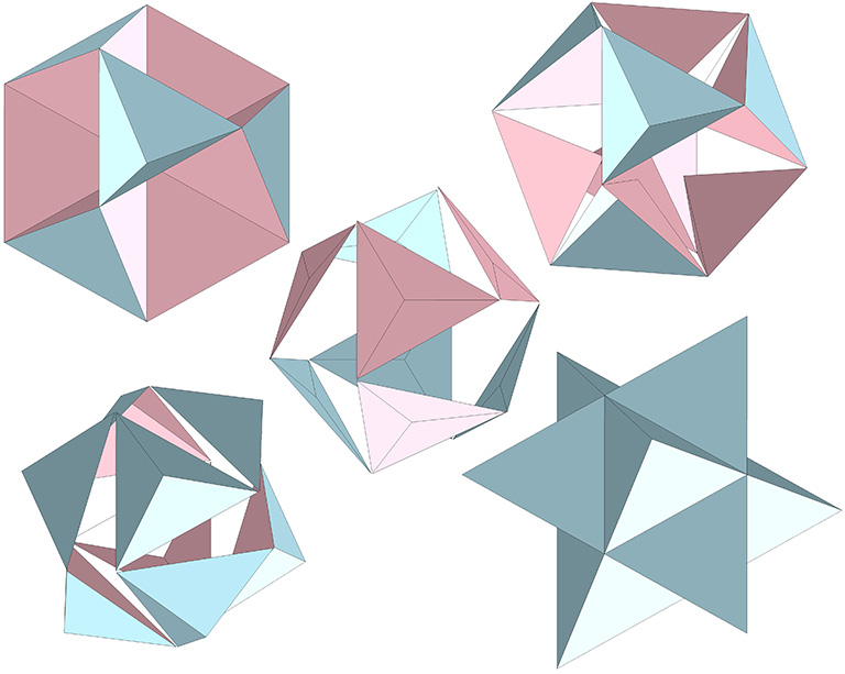
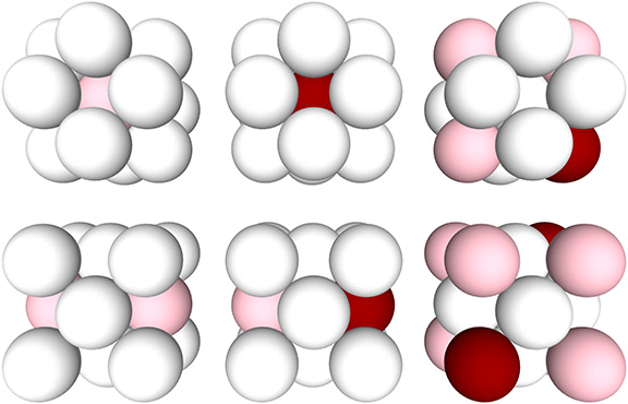
As I said above, radially close-packed spheres divide naturally into vector equilibria and cubes, and we may think of one becoming the other in the jitterbug. In a “crystalized” matrix, we find three variations of each, i.e, three unique VEs and three unique cubes, each with a unique arrangement of the three categories of sphere. These I’m calling “blinkers,” borrowing from the lexicon of the legendary Game of Life which was developed by mathematician John Horton Conway in 1970.
The six “blinkers” of the isotropic vector matrix: A crystalized isotropic matrix produces three unique categories of VE (top row) and three unique categories of the cube (bottom row).
As the matrix jitterbugs, one cube or VE will be replaced with another—different, or the same rotated from its original orientation. They will appear to blink, flash, rotate, and oscillate as spheres are replaced by spaces and the spaces are replaced, again, by spheres. The jitterbug, in effect, can generate an infinite number of patterns that are replicated and regenerated throughout the matrix. In effect, the dull crystal is made into a kind of neural network by this interpretation of the jitterbug transformation.
“The first layer consists of 12 spheres tangentially surrounding a nuclear sphere; the second omnisurrounding tangential layer consists of 42 spheres; the third 92, and the order of successively enclosing layers will be 162 spheres, 252 spheres, and so forth. Each layer has an excess of two diametrically positioned spheres which describe the successive poles of the 25 alternative neutral axes of spin of the nuclear group.” — R. Buckminster Fuller, Synergetics, 222.23
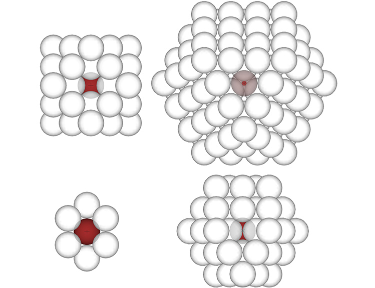
The four sets of 3, 4, 6, and 12 axes that define the 25 great circles of the vector equilibrium also comprise all line-of-sight connections between spheres radially close-packed in the isotropic vector matrix. That is, each axis proceeds directly, without deviation, through interstitial space from one sphere center to the next. This may be made more clear with the following illustration.
Line of site connections between the nucleus (red) and the next sphere on the axis of the set of 3 (top left), 4 (top right), 6 (bottom left), and 12 (bottom right) great circles of the vector equilibrium.
In the above illustration,
The axis for the 3 great circles (top left) connects the semi-transparent sphere in the F2 layer with the nucleus (red), having passed through interstitial space in the F1 layer. Note that this is the only axis that provides a direct connection between nuclei and nuclear voids (see Categories of Spheres in the Isotropic Vector Matrix: Nuclei, F1 Shells, and “Nuclear Voids”). The semi-transparent sphere in the F2 layer will be surrounded by the F1 shells of its surrounding nuclei, and therefore qualifies as a nuclear void.
The axis of the 4 great circles (top right) connects the semi-transparent sphere in the F3 layer with the nucleus (red) after having passed through interstitial space in both the F2 and F1 layers. Note that this is the only axis that provides a direct connection between nuclei; the semi-transparent sphere in the F3 layer will have its own layer of 12 spheres, and therefore qualifies as a nucleus.
The axis of the 6 great circles (bottom left) is unique in that it forms an unbroken chain of spheres in direct contact with one another. The semi-transparent sphere in the F1 shell is in direct contact with the nucleus.
The axis of the 12 great circles (bottom right) connects the semi-transparent sphere in the F2 layer with the nucleus after having passed through what Fuller calls the “kissing point”, i.e., the point of contact between two spheres in the F1 layer.
Set of 3 Great Circles of the VE
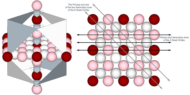
The axes of the 3 great circles pass through the centers of opposing square faces of the VE. Its primary axis connects nuclei in every fourth layer. Their great circle planes are in alignment with the three unique axes for the 3 Great Circles, and two of the three unique axes for the 6 Great Circles.
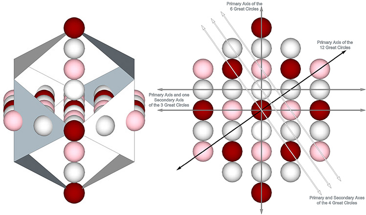
The set of 3 Great Circles is defined by the three axes passing through opposing square faces of the VE (left). The axes define great circle planes (right) on which lie the primary and secondary axes of the the set of 3, and the primary and one secondary axis of the set of 6 Great Circles.
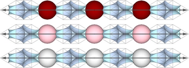
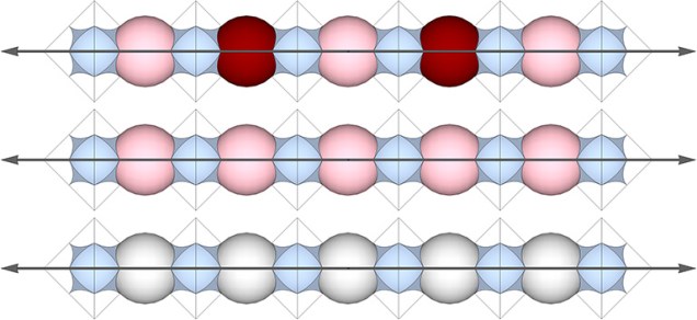
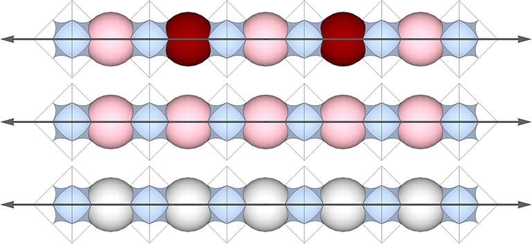
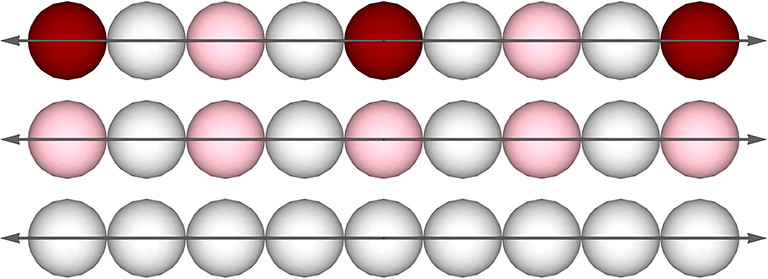
The axes pass alternately through a space (concave VE) and a sphere (convex VE). On the primary axes, the spheres alternate between nuclei (shown in red) and nuclear voids (pink). On the two secondary axes (those that do not pass through a nuclear sphere), the spheres are either all nuclear voids (pink) or spheres that occupy the F1 shells of nuclei. Shell spheres are shown in white. (See: Categories of Spheres in the Isotropic Vector Matrix: Nuclei, F1 Shells, and “Nuclear Voids”.)
The primary axis (top) and the secondary axes (middle and bottom) of the set of 3 Great Circles.
Set of 4 Great Circles of the VE
The axes of the 4 great circles pass through the centers of opposing triangular faces of the VE. Its primary axis connects nuclei in every 3rd layer. Their great circle planes are in alignment with the three unique axes for the sets 6 and 12 Great Circles.
The set of 4 Great Circles is defined by the four axes passing through opposing triangular faces of the VE (left). The axes define great circle planes (right) on which lie the primary and secondary axes of the the set of 6, and the set of 12 Great Circles.
The primary axis joins nuclei. The secondary axes join nuclear voids or shell spheres. Between each sphere on the axes is interstitial space consisting of a space (concave VE) flanked by one positive and one negative interstice (concave octahedra). See: Spheres and Spaces, and; Spaces and Spheres (Redux).
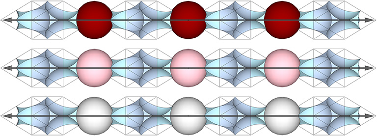
The primary axis (top) and the secondary axes (middle and bottom) of the set of 4 Great Circles.
Set of 6 Great Circles of the VE
The axes of the 6 Great Circles pass through opposing vertices of the VE. Its primary axis connects nuclei in every fourth layer. Their great circle planes are in alignment with the three unique axes of the 4 Great Circles, the primary axis and and one secondary axis of the 3 great circles, and the primary axis of the 6 and 12 Great Circles.
The set of 6 Great Circles is defined by the six axes passing through opposing vertices of the VE (left). The axes define great circle planes (right) on which lie the primary and secondary axes of the the set of 4, the primary and one secondary axis of the set of 3, and the primary axes of the sets of 6 and 12 Great Circles.
The primary axis joins nuclei and nuclear voids between each of which is a shell sphere. One secondary axes joins nuclear voids each separated by a shell sphere, and the other secondary axis forms an unbroken chain of shell spheres.
The primary axis (top) and the secondary axes (middle and bottom) of the set of 6 Great Circles.
Set of 12 Great Circles of the VE
The axes of the 12 Great Circles pass through the centers of opposing edges of the VE. Its primary axis connects nuclei in every fifth layer. Their great-circle planes are in alignment with the three unique axes of the 4 Great Circles, and the primary axis of the 6 Great Circles.
The set of 12 Great Circles is defined by the twelve axes passing through opposing edges of the VE (left). The axes define great circle planes (right) on which lie the primary and secondary axes of the the set of 4, and the primary axis of the set of 6 Great Circles
Primary and secondary axes of the 12 great circles follow the same pattern as the axes of the 6 great circles, but with all all spheres separated by interstitial space.
The primary axis (top) and the secondary axes (middle and bottom) of the set of 12 Great Circles.
Knowing how the three categories of spheres are distributed along the primary axes should enable us to count the total number of nuclei in each shell of the vector equilibrium. The primary axes for the sets of 3 and 6 Great Circles pass through a nucleus with every fourth shell. The primary axis for the Set of 4 Great Circles passes through a nucleus with every third shell And, the primary axes of the set of 12 Great Circles pass through a nucleus with every eighth shell. It follows that only those shells which are multiples of 3, 4 and 8 contain nuclei. The F1, F2, and F5 shells, for example, have none. We also know that nuclei are evenly distributed on a grid of rhombic dodecahedra (see Formation and Distribution of Nuclei in Radial Close-Packing of Spheres), and that the shell growth formula for the rhombic dodecahedron is 12F²+2 (see Concentric Sphere Shell Growth Rates). If anyone knows, or is able to derive the formula, please share.
“Whereas each of the 25 great circles of the vector equilibrium go through the 12 vertexes at least twice; and whereas the 12 vertexes are the only points of inter-tangency of symmetric, unit-radius spheres, one with the other, in closest packing of spheres; and inasmuch as we find that energy charges always follow the convex surfaces of systems; and inasmuch as the great circles represent the most economical, the shortest distance between points on spheres; and inasmuch as we find that energy always takes the most economical route; therefore, it is perfectly clear that energy charges passing through an aggregate of closest-packed spheres, from one to another, could and would employ only the 25 great circles as the great circle railroad tracks between the points of tangency of the spheres, ergo, between points in Universe. We can say, then, that the 25 great circles of the vector equilibrium represent all the possible railroad tracks of shortest energy travel through closest-packed spheres or atoms.” —R. Buckminster Fuller, Synergetics, 458.01
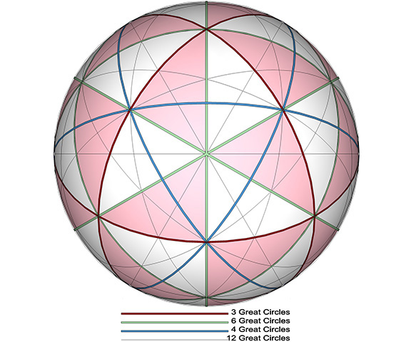
Fuller proposed that the 25 great circles of the vector equilibrium account for all the routes by which energy is transmitted between spheres in the isotropic vector matrix. Or, to put it more dramatically, the great circles defined by the four sets of 3, 4, 6 and 12 spin axes of the VE represent all possible tracks of shortest energy travel between points in the universe.
The four sets of great circles comprising the 25 Great Circles of the Vector Equilibrium (VE). Note the sets of 3 and 6 great circles bound the 48 Basic Equilibrium LCD Triangles, shown in pink and white.
The great circles in the set of 3 are defined by spin axes running through the centers of opposing square faces of the VE. Each great circle passes through four vertices and therefore has four opportunities with each 360° circuit to connect to an adjacent sphere.
On the axis of the 3 great circles, the set of 3 reveals four equally efficient paths, two of which are shown below (left).
On the axis of the 4 great circles, the set of 3 reveals six equally efficient paths, one of which is shown in below (left middle).
All of the great circle sets connect spheres on the axis of the 6 great circles with equal efficiency, differing only in the number of alternate paths; the set of 3 (right middle), reveals two.
On the axis of the 12 great circles, the set of 3 reveals two equally efficient paths, one of which is shown below (right).
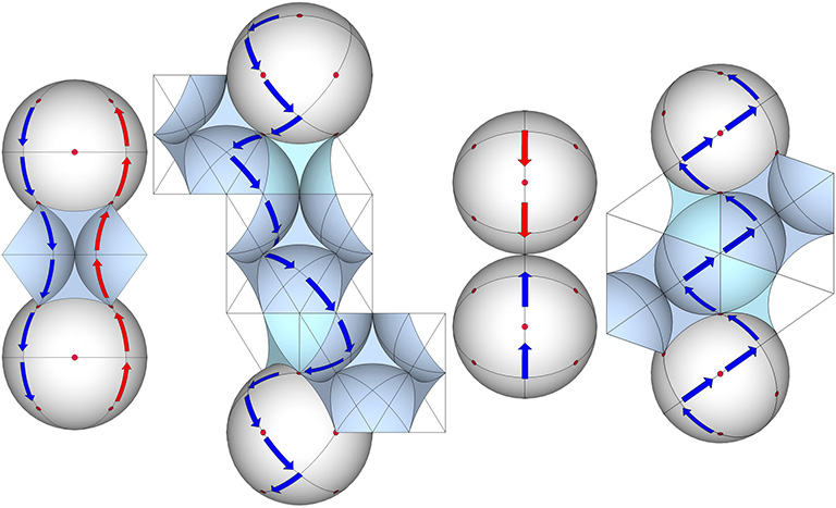
Shortest-distance inter-sphere connections via the set of 3 great circles along the axis of the 3 great circles (left), 4 great circles (left middle), 6 great circles (right middle), and 12 great circles (right).
The Set of 4 Great Circles
The great circles in the set of 4 are defined by spin axes running through opposing triangular faces of the vector equilibrium (VE). Each great circle passes through six vertices and therefore has six opportunities with each 360° circuit to connect with an adjacent sphere.
On the axis of the 3 great circles (top), the set of 4 reveals eight equally-efficient helical routes that complete a cycle every other sphere.
On the axis of the 4 great circles (middle top), the set of 4 reveals eight equally-efficient helical routes the complete a cycle every fourth sphere.
On the axis of the 6 great circles (middle bottom), the set of 4 reveals four equally-efficient routes between spheres.
On the axis of the 12 great circles (bottom), the set of 4 reveals two equally-efficient routes between spheres.
Shortest-distance inter-sphere connections via the set of 4 great circles along the axis of the 3 great circles (left), 4 great circles (left middle), 6 great circles (right middle), and 12 great circles (right).
The Set of 6 Great Circles
The great circles in the set of 6 are defined by spin axes running through opposing vertices of the vector equilibrium (VE). Each great circle passes through two diametrically opposed vertices.
On the axis of the 3 great circles, the set of 6 (left) reveals 4 equally-efficient routes between spheres.
On the axis of the 4 great circles, the set of of 6 (middle left) reveals a branching network of at least 36 equally-efficient paths.
On the axis of the set of 6 great circles, the set of 6 (middle right) reveals two equally-efficient paths between spheres.
On the axis of the 12 great circles, the set of 6 (right) reveals two equally-efficient paths between spheres.
Shortest-distance inter-sphere connections via the set of 6 great circles along the axis of the 3 great circles (left), 4 great circles (left middle), 6 great circles (right middle), and 12 great circles (right).
The Set of 12 Great Circles
The great circles in the set of 12 are defined by spin axes running through the midpoints of opposing edges of the vector equilibrium (VE). As with the set of 6, each great circle in the set of 3 passes through two diametrically opposed vertices.
On the axis of the set of 3 great circles (left), the set of 12 reveals eight equally-efficient routes between spheres.
On the axis of the 4 great circles (middle left), the set of 12 reveals four equally-efficient paths, one of which is shown.
On the axis of the set of 6 great circles (middle right), the set of 12 reveals four equally-efficient paths.
On the axis of the set of 12 great great circles (right), the set of 12 reveals two equally-efficient paths, one of which is shown.
Shortest-distance inter-sphere connections via the set of 12 great circles along the axis of the 3 great circles (left), 4 great circles (left middle), 6 great circles (right middle), and 12 great circles (right).
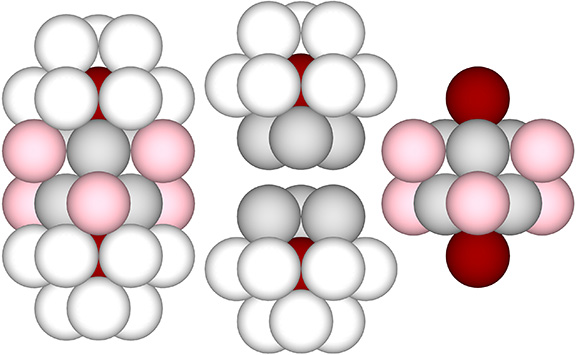
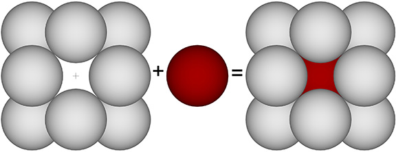
When modeling the distribution of nuclei in the isostropic vector matrix, I distinguish between the nuclei and the 12-sphere shells that isolate and define them. These nuclear domains, each consisting of one nuclear sphere and a 12-sphere shell, defines the vector equilibrium, or VE.
The nuclear domain (right) consists of a 12-sphere shell (left) and the nucleus (center).
Nuclei are distributed in the isotropic vector matrix along the edges and at the centers of rhombic dodecahedra with edge lengths of √6 times the sphere diameter. The edges align with the primary axis of VE’s set of 4 great circles.
Nuclei and their shells do not close-pack to fill all-space. Between these nuclear clusters are gaps which combine to form holes that run laterally through the isotropic vector matrix.
Nuclear domains (the nuclei and their 12-sphere shells) do not close-pack to fill all space. The vacancies form holes that run laterally through the isotropic vector matrix.
The spheres that fill these voids can be isolated to show that they all lie on a cubic grid which follows the square-face diagonals of close-packed F2 VEs.
The voids left in the isotropic vector matrix by close-packed nuclear domains are filled by spheres distributed around each nucleus on the diagonals of a VE with an edge-length of 2 sphere diameters.
I refer to these as “nuclear voids” because, like the nuclei, each occupies the center of a VE, but unlike the nuclei, they do not have their own 12-sphere shells. Rather, every sphere in direct contact with a “nuclear void” is uniquely identified with the shell of one of its neighboring nuclei.
The nuclear void (pink) occupies the center of VE whose vertices are all occupied by the spheres from the shells of neighboring nuclei.