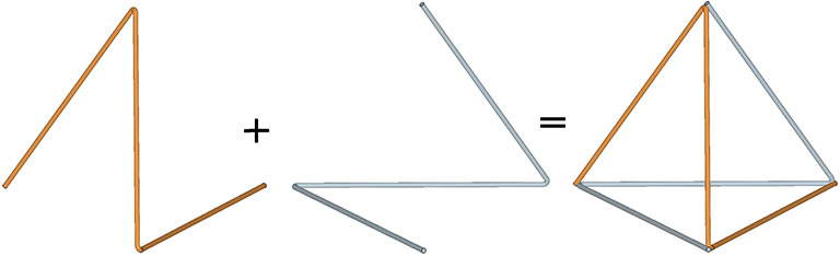
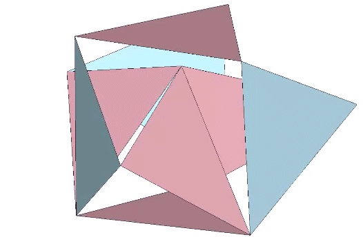
A tetrahedron may be constructed from two open-ended triangles.
Tetrahedron Constructed from Two Open-Ended Triangles
If we use this construction in the isotropic vector matrix, the open ends of each triangle join with similar triangles in the adjacent tetrahedra to form wave patterns that propagate linearly through the matrix, each oriented at 90° to the other. The entire matrix may be built though the duplication of orthogonally paired waves.
Transverse Waves in the Isotropic Vector Matrix
Significant to this model of the isotropic vector matrix is its demonstration of the fundamental principle that no two vectors may pass through the same point simultaneously. All vertices in the matrix redirect their vectors, rather than act as focal points for their convergence.
Deflecting Vectors at Vertices of the Transverse Wave Model of the Isotropic Vector Matrix
For each of the six axes of the isotropic vector matrix, i.e., the six vertex-to-vertex axes of spin of the vector equilibrium, there are four unique waves, two running clockwise and two running counter clockwise on either side of the axis, for a total of 24 (6×4) waves converging on and deflecting from every point.
For each of the six axes of the isotropic vector matrix, i.e., the six vertex-to-vertex axes of spin of the vector equilibrium, there are four unique waves, two running clockwise and two running counter clockwise on either side of the axis.
Note that the axis that defines the linear orientation of the wave is excluded from the wave itself which traces a path along three of the remaining five edge vectors of the tetrahedron. The clockwise and counter-clockwise waves of the positive and negative tetrahedra each share one leg oriented at 90° to the wave’s directional axis, underscoring the polarization of the pair.
The six axes of the isotropic vector matrix define the six edges of the tetrahedron. The waves from these six axes wrap around each tetrahedron such that each of its six edges includes a leg from four separate waves.
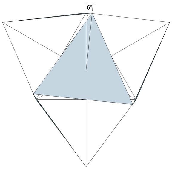
The neutral axes of six chains of open-ended equilateral triangles intersect to form a regular tetrahedron with four vectors per edge.
This recapitulates the quadrivalent (four vectors per edge) tetrahedron that results when the jitterbug is given an extra 180° twist.
With a 180° twist, the jitterbugging VE can be collapsed into a regular tetrahedron with four vectors per edge.
This wave pattern can also be modeled with continuous ribbons of equilateral triangles which are then folded at the same angles as the three vectors of the open-ended triangle above.
The isotropic matrix modeled by the folding of a linear ribbon of equilateral triangles mirrors the transverse wave model of open-ended triangles.
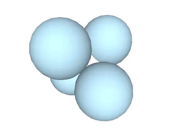
The octahedron can be constructed from four open-ended triangles.
Four open-ended equilateral triangles combine to form the regular octahedron.
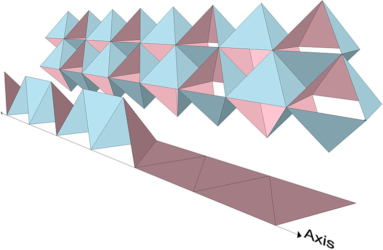
The open-ended triangles of the octahedron may be joined in parallel linear waves that form a continuous chain of octahedra.
The open-ended triangles of the octahedron joined in four parallel linear waves forming a continuous chain of octahedra.
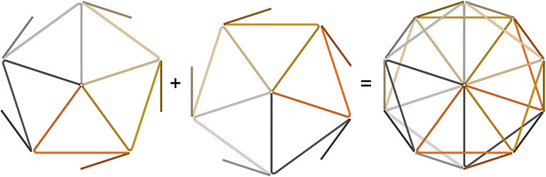
The icosahedron can be constructed from ten open-ended triangles.
Ten open-ended equilateral triangles combine to form the regular icosahedron.
There are numerous ways of joining the open-ended triangles of the icosahedron end-to-end, but all form wave-dispersal patterns in which the icosahedron appears never to repeat.
Joining the open-ended triangles of the regular icosahedron forms a wave-dispersal pattern that appears to never repeat the original icosahedron.
“The geometrical model of energy configurations in synergetics is developed from a symmetrical cluster of spheres, in which each sphere is a model of a field of energy all of whose forces tend to coordinate themselves, shuntingly or pulsatively, and only momentarily in positive or negative asymmetrical patterns relative to, but never congruent with, the eternality of the vector equilibrium. […] Synergetics is comprehensive because it describes instantaneously both the internal and external limit relationships of the sphere or spheres of energetic fields; that is, singularly concentric, or plurally expansive, or propagative and reproductive in all directions, in either spherical or plane geometrical terms and in simple arithmetic.” — R. Buckminster Fuller, Synergetics, 205.01
The point in conventional geometry is replaced by the sphere in Fuller’s geometry. Vertices are the geometric centers of spheres, and vectors connect sphere centers. There are no continuous lines. Surfaces and volumes are point populations, i.e., close-packed spheres or the vertices that define the sphere centers. The minimum point is defined as a vector equilibrium (VE) of zero frequency, i.e. the nuclear sphere. The shell volume of the zero-frequency VE is give by the shell-growth formula for radially close-packed spheres, 10F²+2, as “2,” i.e., the inside surface, plus the outside surface. Unity is plural and at minimum two.
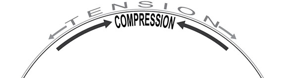
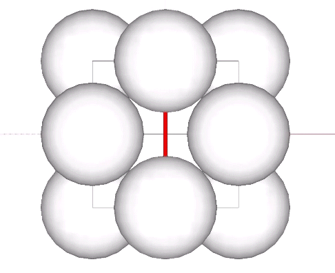
Every sphere has two surfaces, one convex and the other concave. The concave (interior) surface resists compressive forces while the convex (exterior) surface resists tensile forces.
Bending pressure results in tension along the outside of the curve, and compression along the inside of the curve.
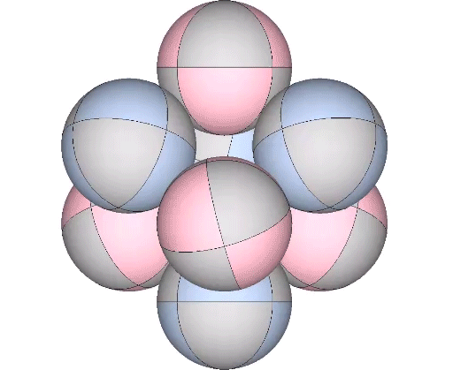
In the following illustration, cutaways of the sphere show the concave interior surface (pink) under compression, and the convex exterior surface (blue) under tension.
A sphere holds its shape by balancing the tensile forces of its outer surface (blue) with the compressive forces of it inner surface (pink).
These two forces can be modeled as the radials and circumferential vectors of the vector equilibrium (VE). In the following illustration the radials are represented by rigid struts which resist the compressive force provided by the circumferential vectors represented by elastic bands which in turn resist the tensile force provided by the rigid struts.
The tensile forces of the circumferential vectors of the VE (blue) are balanced by the compressive forces of its radial vectors (brown).
The tensegrity model clearly represents the inter-dependence of the two forces, with the convex tension represented by continuous tendons, and the concave compression represented by the discontinuous struts.
The tensile forces of the 6-strut tensegrity’s continuous tendons are balanced by the compressive forces of its discontinuous struts
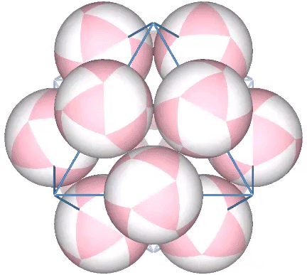
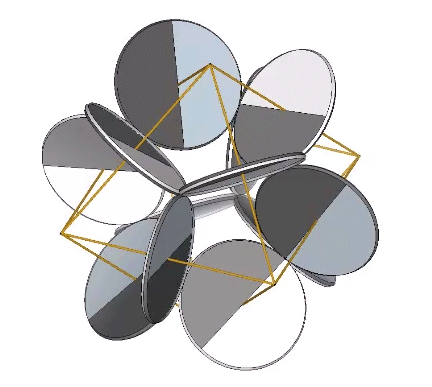
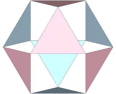
In the bow tie model, concave and convex are disclosed as opposite sides of the four great-circle disks that comprise the spherical VE. The combined surface areas of the four disks is the same as the surface area of the sphere they describe. In the illustration below, the two sides are distinguished by color, one pink and the other blue.
In this model of the vector equilibrium (VE), the inside and outside surfaces of the sphere are disclosed as opposite sides of four great-circle disks folded into bow-ties. Their combined surface areas exactly equals the surface ares of the sphere they describe.
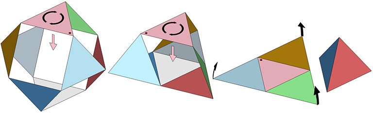
In the quanta model, the two forces are represented by the integrative A modules and the dis-integrative B modules. The close packed spheres and spaces which exchange places in the jitterbug, are represented by two rhombic dodecahedra, one being the inside-out version of the other.
The quanta-module construction of the rhombic dodecahedron models the transformation between spheres or spaces in the isotropic vector matrix by turning itself inside out.
The first of the two rhombic dodecahedra has at its core a concave octahedron made entirely of B modules. This core is completely enveloped by A modules, first forming a regular octahedron, and then the rhombic dodecahedron. It suggests an implosive, integrative event.
Quanta module construction of a space.
The second of the two rhombic dodecahedra exposes all of its modules, both A and B, on its surface. None are entirely contained by the others, and it suggests an explosive, dis-integrative event.
Quanta module construction of a sphere.
In the jitterbug transformation of the quanta model, the two rhombic dodecahedra exchange places, suggesting one is the explosive space (the expanding octahedron) which takes the place of the imploding nucleus (the contracting VE). This concept may be more clear if we look at the transformations of the core in isolation from the shell.
The core of the the two quanta module constructions of the rhombic dodecahedron. The B quanta modules point outward (sphere) or inward (space).
The B modules are arranged in arrow-like shapes that point their faces inward in the transformation from VE to octahedron (contracting nuclei), and outward in the transformation from octahedron to VE (expanding spaces). Fuller’s intuitions about the energy characteristics of the two modules, entropic for the B quanta modules, syntropic for the A quanta modules, seem all the more inspired the more deeply we look into the geometry.
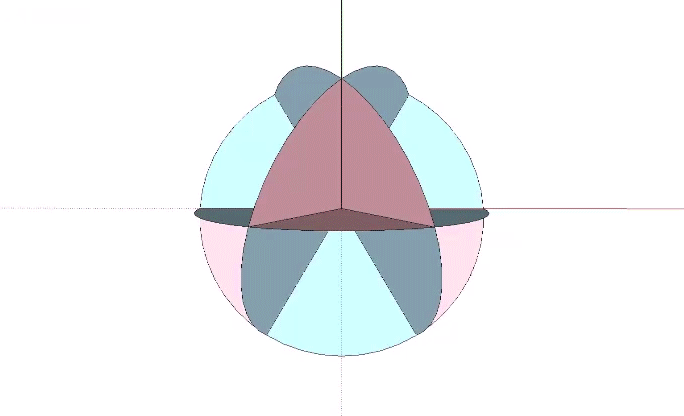
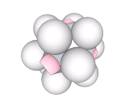
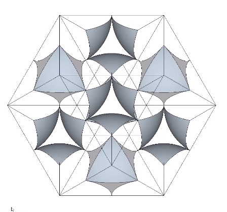
In the interstitial model of the isotropic vector matrix (see Spaces and Spheres Redux), the two forces are made self-evident in the literal exposure of the of the concave interior and convex exterior surfaces of the spheres, represented here as blue concave VE “spaces”, gray convex VE spheres, and pink concave octahedra interstices.
The interstitial model of the isotropic vector matrix exposes the concave inside surfaces of the spheres, as well as the four great circles of the vector equilibrium whose vertices are the points of contact between adjacent spheres.
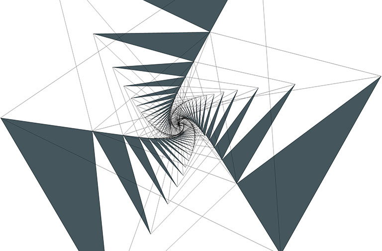
I stumbled across a rigid structure that seems to be a cross between a tensegrity prism, a polyhedron, and a tetrahelix.
Eight vertex-bonded equilateral triangles arranged into structural helix with a twist of six degrees per module.
I find it curious because a) it doesn’t seem to conform to the triangulation rule for rigid structures, b) it looks like it ought to be tensegrity prism, but it isn’t obvious which of the vectors can be replaced with tendons, and c) the top and bottom triangles are twisted at exactly six degrees, or 1/60th of a full 360° cycle.
In each module of the structural helix, the top triangle is rotated six degrees from the bottom triangle
Stacking one on top of another is also quite beautiful.
Top view of the helix constructed from twenty modules with a combined rotation of 120 degrees.
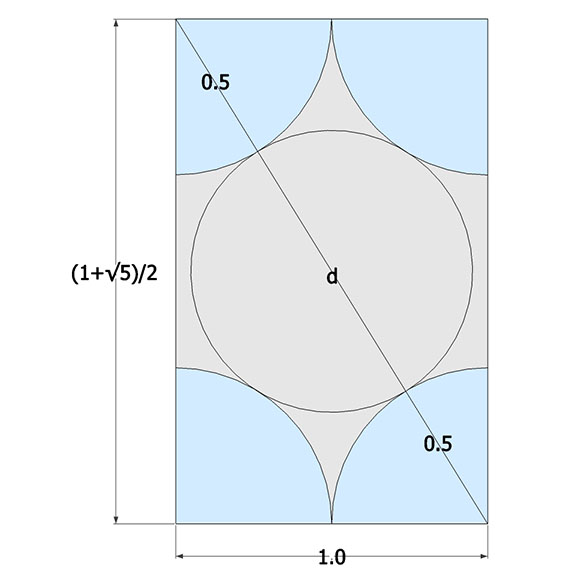
If a spherical nucleus were at the center of a close-packed array of spheres in the icosahedron configuration, what would be its radius? That is, by how much must the nucleus shrink when the close-packed array jitterbugs from the VE to the icosahedron? Knowing that the icosahedron can be constructed from the three golden rectangles arranged orthogonally around a common center, it’s a simple matter of trigonometry.
The regular icosahedron can be constructed from three intersecting golden rectangles.
The diagonal, d, of the regular icosahedron is equal to the diagonal of the golden rectangle from which it is constructed. The diameter for the center circle is d-1.
The diagonal (d) is the the square root of the sum of the squares of the two sides, or √(((1+√5)/2)+1²) ≈ 1.902113:
The diameter of the nucleus at the center of an icosahedron made up of unit-radius spheres is the length of the diagonal minus 1, or approximately 0.902113.
The golden ratio has some curious properties. For example, its square is equal to itself plus one:
Knowing this, we can reduce the expression under the radical above to ((1+√5)/2)+2:
Since the expression on the left is the golden ratio, it follows that the diagonal of the icosahedron may be expressed as √(2+φ):
The isotropic vector matrix can be modeled as vectors, struts and tendons, quanta modules, or as spheres and their interstices. All these models originated in Fuller’s geometry with the close packing of unit-radius spheres—ping-pong balls or Styrofoam spheres he glued together. We may be tempted to think of these spheres, as we used to the think of atoms, as solid and indivisible. But by now we should be accustomed to thinking of these fundamental particles as divisible into obscure quanta with strange properties, as clouds of energy, or as waves in a quantum field. So it may not bother us to see these otherwise solid spheres merging and diverging in the spherical model of the jitterbug.
The jitterbug as a single VE with its vertices represented by unit spheres.
But if we think of the spheres as quanta, their number, by fundamental conservation laws, should remain constant throughout the jitterbug. If we assume one sphere per vertex, what is the ratio of vertices in the isotropic vector matrix compared to the matrix at tensegrity equilibrium? The former includes the nuclei which are replaced by the six struts in the tensegrity model. But it does not appear that those make up for the increase in the number of vertices, i.e. shell vertices plus nuclei in the vector model do not add up to the number of vertices in the tensegrity model. Where do the extra spheres/vertices come from?
Fuller thought the vectors, whose length defines the sphere diameter, were a constant in the jitterbug. But it appears that the true constant in the jitterbug is the length of the diagonal, i.e. the length of the struts in the tensegrity model. If we hold the strut length constant, the spheres do not fully divide in the icosahedron phases of the jitterbug. When the jitterbug is conceived as an unbounded matrix, the spheres never divide without simultaneously merging with neighboring spheres (which are also dividing).
The partial division of the spheres that reaches its maximum at the Jessen phase, i.e., at tensegrity equilibrium, might be conceived as the counterpart to the separation of tension and compression in the tensegrity model. That is, the spheres’ convexity (tension) and concavity (compression) are being isolated in the same way that the tendons (tension) and struts (compression) are isolated in the tensegrity model.
The jitterbug, oscillating into and out of tensegrity equilibrium. Note that maximum division of the spheres occurs between, not at, the vector equilibrium phases.
In the figure below, this division of spheres into the convex and concave counterparts is represented by green spheres dividing (partially) into blue and yellow spheres, and then recombining into green spheres.
Three phases of the jitterbug represented as unit spheres (top), as spaces and interstices (bottom left and right), and by six-strut tensegrity spheres (bottom middle). The green spheres partially divide into blue and yellow spheres in the icosahedron phases of the jitterbug (top middle. Each blue-yellow pair constitutes one sphere.
Isotropy is restored when the VE contracts into an octahedron and when the octahedron expands to the VE. But in between, when both shapes describe regular or irregular icosahedra, the only constant is the strut length which (if the vectors at equilibrium are of unit length) is equal to √2, the diagonal of the unit-edged cube.
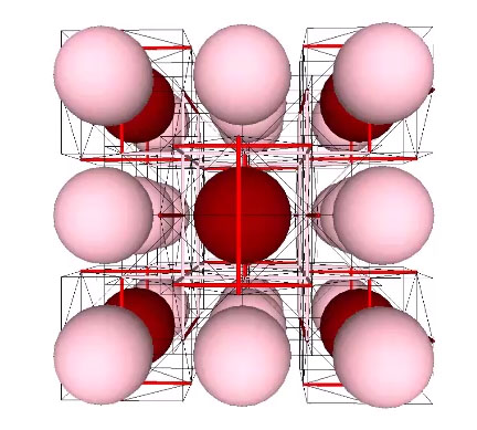
The increase in the number of vertices is modeled in the tensegrity model of the jitterbug as the merging and diverging of struts. The struts, like the spheres, are doubled up at vector equilibrium, and do not quite fully separate at tensegrity equilibrium. In the figure below, the nuclei in the sphere model have been superimposed onto the tensegrity matrix at vector equilibrium. The red nuclei are associated with 12-sphere shells unique to that nucleus. The pink nuclei share their 12-sphere shells with the surrounding nuclei. (See Formation and Distribution of Nuclei in Radial Close-Packing of Spheres.)
The distribution of nuclei superimposed onto the tensegrity model at vector equilibrium.
To see how the struts in the tensegrity model serve the same purpose as the nuclei in the sphere model, imagine the tensegrity jitterbug with the struts squeezed together into the octahedron configuration. As the struts separate, imagine unit-radius spheres centered at each of their ends. They start out as porous clouds but harden into impenetrable spheres just as the struts have separated into the VE configuration. The tensegrity-plus-spheres model is at equilibrium, with the spheres and struts both supplying compression resistance to the tension web of tendons. The de-nucleated sphere shell will not collapse into an icosahedron as long as the struts remain rigid.
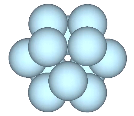
The tensegrity model at vector equilibrium, when coupled with the spheres model, holds the spheres in the same 12-around-1 configuration as radially close-packed spheres around a common nucleus.
This model underscores Fuller’s proposition that gravity is a 90° precessional effect. That is, mass-attraction is modeled here by the tension web, the chords between the sphere centers which are situated at right angles to the radial vectors which would otherwise connect each to their common nucleus. The nucleus of the radially close-packed spheres model has here been replaced with the struts of the tensegrity model.
If we close-pack 12 spheres around a central nucleus and then remove the central sphere, the remaining spheres are free to rotate along twelve axes perpendicular to the radii connecting the sphere centers with their common center. The combined axes describe the regular octahedron.
With the nuclear sphere removed, the surrounding twelve spheres rotate freely as synchronous gears
We can also replace the spheres by wheels, which is mesmerizing, though perhaps not very helpful to conceptualizing the geometry.
De-nucleated VE with spheres reduced to disks
The effect is related to, but not identical with the jitterbug. Both are related to the removal of the nucleus, but with the jitterbug, there are only four axes of spin, and these are identical with, rather than perpendicular to, the radii.
The classic model of the jitterbug
This is perhaps made more clear if we replace the eight triangles of the classic model of the jitterbug with eight wheels rotating synchronously on the four radial axes of the cube.
The eight triangles of the classic model of the jitterbug replaced with wheels rotating on the four radial axes of the cube.
The eight wheels may be replaced with spheres.
The eight triangles of the classic model of the jitterbug replaced with spheres.
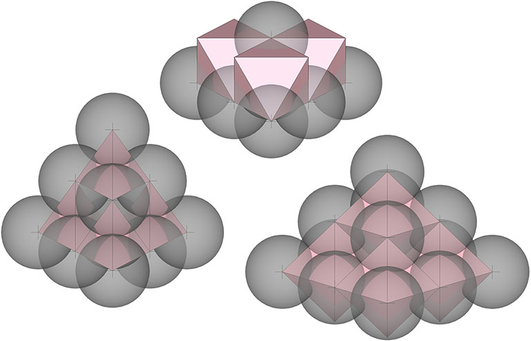
It may seem that there are at least three ways of stacking cannonballs, i.e., from a triangular base to form a pyramid with three sides; from a square base to form a pyramid with four sides; or as a shallow 3-sided pyramid.
The three standard methods of stacking unit-radius spheres: regular tetrahedron (left); one-quarter tetrahedron (center); and one-half octahedron (right).
All three methods of stacking unit-radius spheres are really just different ways of looking at the single method of the radial close-packing of spheres around a central nucleus.
The jitterbug transformation is conventionally modeled as hinged vectors and rotating triangles. But as the vertices are meant to model sphere centers, I’ve here replaced the vertices of the vector equilibrium (VE) with spheres.
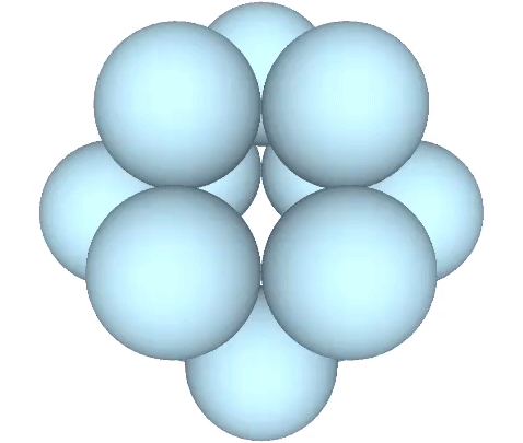
Twelve unit-radius spheres close pack around a central nuclear sphere in the shape of the vector equilibrium (VE).
The doubling up of edges at the octahedron phase in the vector model of the jitterbug is represented in the sphere model of the jitterbug by merging and diverging unit-radius spheres. Different views and rotations of the model reveal some interesting characteristics of the transformation. If the view is synchronized with the rotation of the top and bottom triangles, the transformation resembles a pump with spheres orbiting around its equator.
Sphere model of the jitterbug with top and bottom triangles fixed and viewed perpendicular to the equator.
With the view perpendicular to one of the square faces of the VE, and without rotation, the spheres merge and diverge at right angles.
Sphere model of the jitterbug viewed perpendicular to one of the VE’s square “faces”.
With the view perpendicular to a fixed triangular face, the remaining spheres rotate around the equatorial axis.
Sphere model of the jitterbug viewed perpendicular to a fixed triangular “face”.
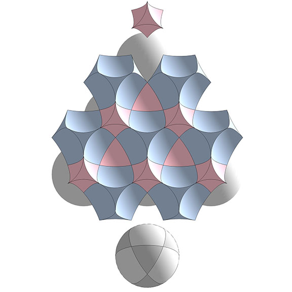
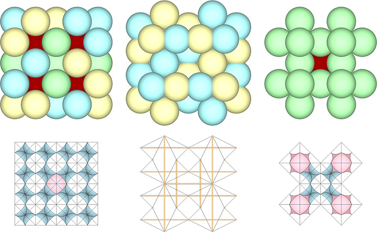
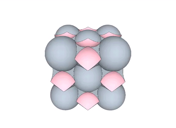
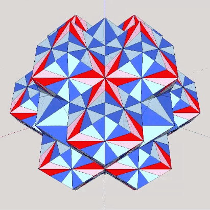
The isotropic vector matrix can be modeled as spheres, vectors, tensegrities, space-filling polyhedra, or as the concave polyhedra occupying the spaces and interstices between radially close-packed spheres. The space between radially close-packed spheres is a continuous web of concave octahedra and concave vector equilibria (VEs).
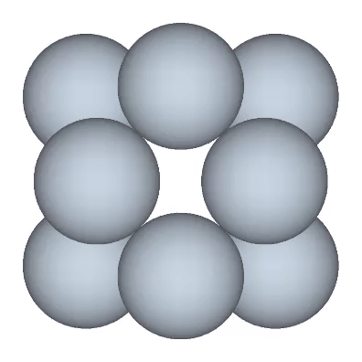
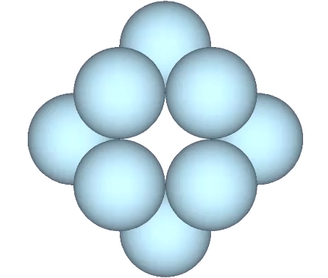
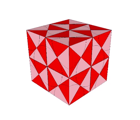
Six spheres close-packed as octahedra surround a nuclear space (“Space”) in the shape of a concave VE, whose volume is slightly less than 1/3 that of the sphere, and slightly more than 1/3 that of the octahedron. The following volumes are all measured in unit tetrahedra. See Areas and Volumes in Triangles and Tetrahedra.
The tetrahedral volume of the concave VE space at the center of six close-packed unit-diameter spheres is the volume of the unit octahedron (4) minus the the volumes of six 1/10 spheres.
Volume of concave VE “space” = 4 – 3π√2/5 ≈ 1.334270237 ≈ 33.356755928% the volume of the unit octahedron ≈ 33.298224115% the volume of the unit-diameter sphere
Concave VEs define the “spaces” at the centers of octahedra in the isotropic vector matrix.
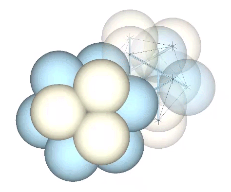
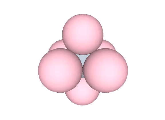
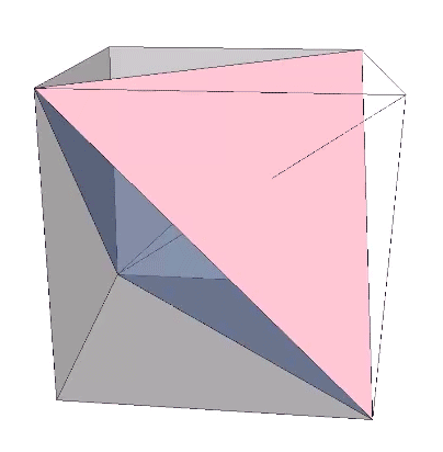
Four spheres close-packed as tetrahedra surround an interstitial space (“Interstice”) in the shape of a concave octahedron, whose volume is a little more than 11% that of the tetrahedron, and a little more than 2.5% that of the sphere.
The tetrahedral volume of the concave octahedron interstice at the center of four close-packed unit-diameter spheres is the volume of the unit tetrahedron (1) minus the the volumes of four 1/20 spheres.
Volume of concave octahedron “interstice” = 1 – π√2/5 ≈ 0.111423412 ≈ 11.1423412% the volume of the tetrahedron ≈ 2.5079079% the volume of the sphere
Concave octahedron define the “interstices” between spheres arranged as tetrahedra in the isotropic vector matrix.
The space-to-sphere ratio of the VE is about 44.5/55.5
(6 × volume of concave VE) + (8 × volume of concave octahedron) ≈ 8.00562+ 0.89139 ≈ 8.89701 ≈ 44.485043608% the volume of the VE (20) ≈ 25.031631616% the the volume of the VE’s circumsphere (volume about 35.543)
The space between radially close-packed spheres in the isotropic vector matrix is defined by concave VEs and concave octahedra.
The space-to-sphere ratio of the cube is about 31.5%
(5 × volume of concave VE) + (8 × volume of concave octahedron) ≈ 6.67135 + 0.89139 ≈ 7.56274 ≈ 31.51142% the volume of the cube (volume 24)
The space between the close-packed unit spheres constituting the cube is defined by twelve concave VEs and six concave octahedra surrounding a nuclear concave VE space.
In the jitterbug transformation, the spheres and spaces exchange places. The concave VEs become convex VEs (and vice versa) in a transformation that can be described as turning themselves inside-out.
In the jitterbug transformation, spheres and spaces exchange places by turning themselves inside-out.
When modeled in quanta modules, the exchange takes place between the two distinct constructions of rhombic dodecahedra, the one found at the center of the VE (the sphere, or convex VE), and the other at the center of the octahedron or cube (the space, or concave VE).
The sphere-to-space, space-to-sphere inside-outing of the jitterbug transformation modeled with the two quanta-module constructions of the rhombic dodecahedron.
The jitterbug transformation can also be described by the polarity reversal of the tetrahedra. This is manifested in the vector model by the two tetrahedra, one positive, and one negative, that the rotating triangle in the jitterbug alternately describes.
An isolated triangle from the vector model of the jitterbug transformation alternately defining a positive and a negative tetrahedron.
The polarity reversal of the tetrahedron may be modeled as a 90° rotation. Each tetrahedron is rotated ninety degrees in the transition between the VE and octahedron phases, turning their respective concave octahedron into orientations that describe either a sphere or a concave VE space at their common center.
The polarity reversal of the tetrahedra modeled by their 90° rotations in the interstitial model of the jitterbug.
Again, this correlates beautifully with the quanta-module model. Eight quanta-module cubes (each containing a tetrahedron) are rotated 90° to alternately reveal one of the two quanta-module constructions of the rhombic dodecahedron at their common center—one representing the sphere, and one representing the space.
The polarity reversal of tetrahedra in the jitterbug transformation modeled by the 90° rotation of cubes in the quanta-module model of the jitterbug.
Because the concave octahedron interstices remain constant when the spheres and concave VE spaces exchange places in the jitterbug transformation, their volumes cancel out, and the sphere-to-space ratio of the isotropic vector matrix as a whole is identical with the ratio of volumes of the sphere and concave VE space. That is, the ratio of space to sphere is approximately 2:3.