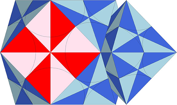
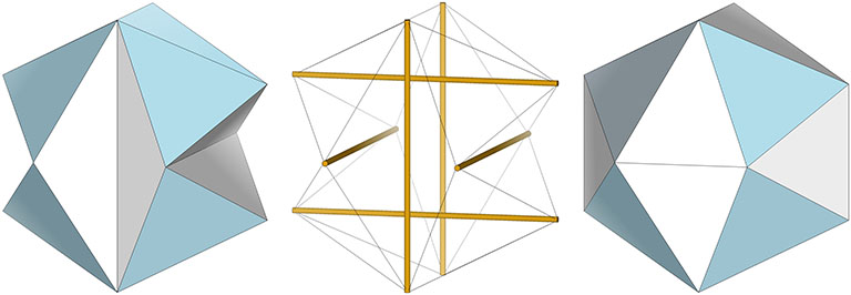
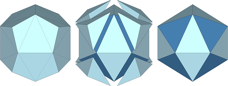
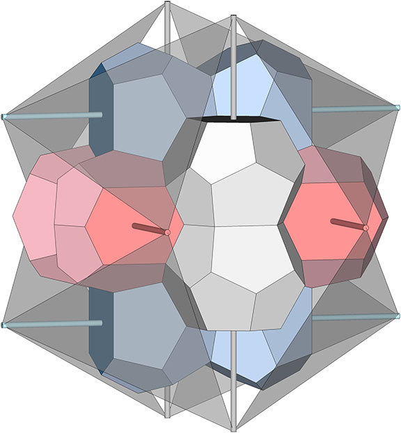
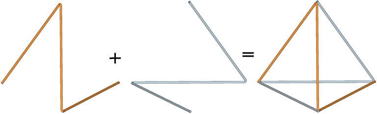
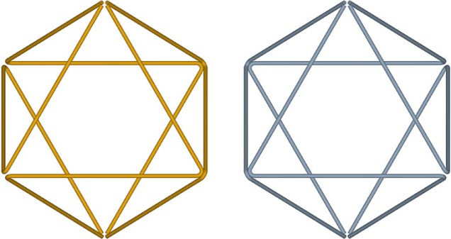
The Jessen Orthogonal Icosahedron (center) constructed from two overlapping VEs (left and right). Click on image to open animation in new tab.
This is halfway between the nuclear sphere at the center of the VE and the space at the centers of its constituent octahedra. The location is apt, as the Jessen marks the halfway point in the jitterbug transformation between the VE and octahedron, i.e., between spheres and spaces.
The Jessen Orthogonal Icosahedron (blue) occupies a position in the isotropic vector matrix diametrically halfway between the spheres and spaces at the centers of VEs and octahedra in the isotropic vector matrix.
The Jessen has a rational tetrahedral volume. (See Jessen Orthogonal Icosahedron and Tensor Equilibrium.) If we attempt to isolate the space it occupies in the quanta module construction of the isotropic matrix, we discover that it can almost, but not entirely be modeled in A and B quanta modules.
The position of the Jessen Orthogonal Icosahedron in the quanta module construction of the isotropic matrix. Click on lower image to open animation in new tab.
At the center of the quanta module construction of the Jessen is the eight-Mite coupler that joins spheres with spaces.
An eight-Mite coupler lies the center of the Jessen Orthogonal Icosahedron, shown here as the six-strut tensegrity sphere whose struts and tendons define the Jessen’s edges. Click on image to view animation in new tab.
Note that the coupler is polarized and seems to point, forwards and backwards, along the vector of its displacement between the VE and octahedron, i.e. from the sphere in the direction of its adjoining space (or vice versa). The only other polyhedron whose quanta module construction is similarly polarized is the cube. The orientation of the cube in the quanta module construction of the isotropic vector matrix determines the polarity of the tetrahedron, and the six-strut tensegrity that defines the Jessen is the spherical phase of the tensegrity tetrahedron, the wave function, if you will, that collapses into either a positive or negative tetrahedron. (See also: Dual Nature of the Tetrahedron.)
“Transformation of Six-Strut Tensegrity Structures: A six-strut tensegrity tetrahedron can be transformed by changing the distribution and relative lengths of its tension members to the six-strut icosahedron [Jessen Orthogonal Icosahedron]. A theoretical three-way coordinate expansion can be envisioned with three parallel pairs of constant-length struts in which a stretching of tension members is permitted as the struts move outwardly from a common center. Starting with a six-strut octahedron, the structure expands outwardly going through the icosahedron phase to the vector-equilibrium phase. When the structure expands beyond the vector equilibrium, the six struts […] lose their structural function (assuming the original distribution of tension and compression members remains unchanged). As the tension members become substantially longer than the struts, the struts tend to approach relative zero and the overall shape of the structure approaches a super octahedron.” —R. Buckminster Fuller, Synergetics, 725.02
Fuller recognized that the six-strut tensegrity structure (which he often referred to as the “tensegrity icosahedron”) and the polyhedron that we are here calling the Jessen Orthogonal Icosahedron, was actually a transformation of the tensegrity Tetrahedron. As I’ve said elsewhere, all that can be reasonably called “structure” in the universe is, fundamentally, a self-supporting integrated system of continuous tension and discontinuous compression that Fuller termed, Tensegrity.
The Jessen Orthogonal Icosahedron represents the spherical, or what I’m calling the “tensor equilibrium” phase, of the tetrahedron. It occurs at the halfway point in the transformation by which the tetrahedron reverses itself, from its positive (clockwise) to its negative (counter-clockwise) state and vice versa. (See illustration below.) The tetrahedron may be unique in this ability. See Dual Nature of the Tetrahedron.
The 6-strut tensegrity is the spherical phase of the tensegrity tetrahedron, seen here transforming to either a positive or a negative tetrahedron.
Approximately midway between its vector-equilibrium phases, the jitterbug describes the regular icosahedron. The collapsing VEs and expanding octahedra, however, do not simultaneously describe the regular icosahedron. The common shape, precisely midway between the transformation from one to the other, is actually the shape of the six-strut tensegrity sphere. This is the “tensor equilibrium” phase of the isotropic vector matrix, in contrast to the more familiar “vector equilibrium” phase.
Precisely midway through the jitterbug transformation, the isotropic vector matrix reaches tensor equilibrium; the contracting VEs and the expanding octahedra oscillate between their vector equilibrium phases and simultaneously describe the shape of the 6-strut tensegrity sphere, or “Jessen Orthogonal Icosahedron.”
Fuller neglected to give the shape a name, perhaps failing to appreciate its full significance. Other mathematicians, namely Borge Jessen, have taken credit for its “discovery,” and Wikipedia affirms its identity as the Jessen Orthogonal Icosahedron.
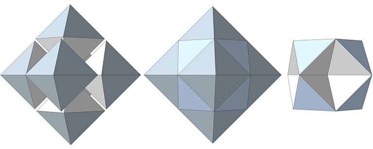
The Jessen Orthogonal Icosahedron (left) describes the shape of the 6-strut tensegrity sphere (center); its concave faces may be replaced with convex faces by rotating their shared base vector 90° and connecting the vertices of their short diagonal (right).
Tensor equilibrium is made intuitively obvious with a physical model of the six-strut tensegrity sphere constructed of rigid struts and elastic tendons.** By pulling apart or squeezing together any one pair of opposing struts, the whole structure symmetrically expands and contracts, i.e. “jitterbugs” between the vector equilibrium states of the VE, at maximum separation, and the octahedron, when each strut pair is bunched together. Between these two maximally stressed states is the Jessen orthogonal icosahedron, or six-strut tensegrity sphere, the unstressed state about which the tensegrity oscillates.
Pulling apart or squeezing together any one pair of opposing struts transforms the six-strut tensegrity causes the others to likewise expand and contract, i.e., to “jitterbug” between the VE and Octahedron.
The tensor equilibrium state is also physically and convincingly demonstrated with the models in the following illustration.
Physical models demonstrating tensor equilibrium include, left to right: the 6-strut tensegrity with the tension web replaced with elastic slings; elastic loops stretched between a cubic scaffold with frictionless rings; the conventional model of the six-strut tensegrity with its continuous tension web; and the Jessen Orthogonal Icosahedron on the far right.
The model on the left is the six-strut tensegrity sphere with its continuous web of tension replaced by rubber-band slings. Second from left is a model built with elastic loops stretched between the edges of a cubic scaffold with frictionless rings. Second from right is the conventional model of the six-strut tensegrity sphere. All of these models slip naturally into their equilibrium state which conforms precisely to the shape of the Jessen Orthogonal Icosahedron on the far right.
** For detailed instructions for constructing these and other models relevant to Fuller’s geometry, see the page, Model Making, on this web site.
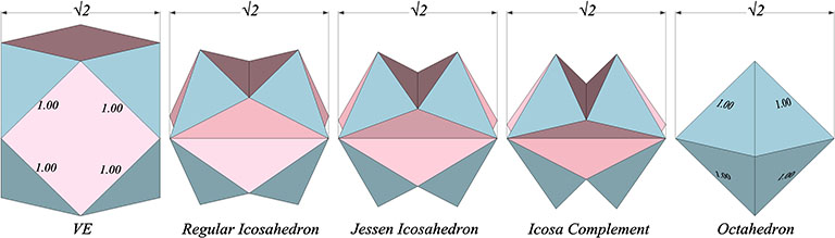
If the long edges of the Jessen’s concave faces are imagined to be the struts of the the six-strut tensegrity sphere, their length would be the square root of two (√2) — the same as the diagonal of the square face of the unit-edge VE and the circumsphere diameter of the unit-edge octahedron. Given a strut length of √2, the Jessen has a rational tetrahedral volume. If the struts are taken to be of unit length, the Jessen has a rational cubic volume.
The phases of the jitterbug transformation with the strut length (long edge of the concave icosahedra) held constant at √2.
If the strut length (d) is taken to be √2,
the concave Jessen’s tetrahedral volume is exactly 7.5, and;
the convex Jessen’s tetrahedral volume is exactly 10.5.
If the strut length (d) is taken to be of unit length (1.00),
the concave Jessen’s cubic volume is exactly 5/16, and;
the convex Jessens cubic volume is exactly 7/16.
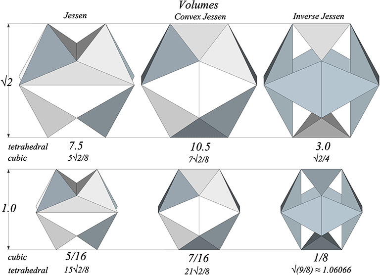
Volumes of the Jessen represented in its concave and convex forms (first and second columns) and as the volumetric difference between the two (right column). Note the tetrahedral volumes are rational when the strut length (long concave edge) is held constant at √2, and that the cubic volumes are rational with the strut length (long concave edge) is held constant at unit length.
The polyhedral form of the Jessen can be represented as six irregular tetrahedra occupying the Jessen’s concavities (right column in the above illustration). With the length of their long edge (strut) equal to √2 their combined tetrahedral volume is 3, the same tetrahedral volume as the unit-diagonal cube. With a unit strut length (d=1), their cubic volume is 1/8, and their tetrahedral volume is, significantly, exactly the value of Fuller’s “Synergetics Conversion Constant,” √(9/8), approximately 1.066066. See Pi and the Synergetics Constants.
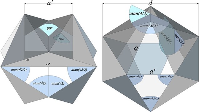
“Orthogonal” refers to the Jessen’s definitive concave form in which its dihedral angles are all 90°; that is, all of the Jessen Orthogonal Icosahedron’s faces meet at right angles. In the Jessen’s convex form, the cosine of one dihedral is the second root of the other: acos(-3/5), and; acos(-√(3/5)), which seems somehow significant.
Dihedral and surface angles of the concave (left) and convex (right) Jessen.
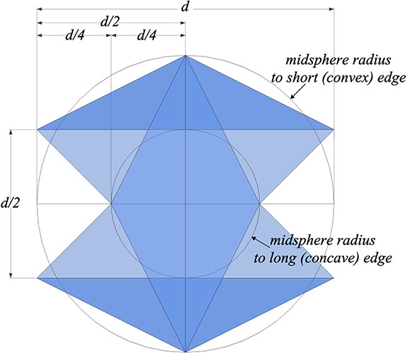
The smallest radius of the Jessen is the midsphere radius to its long (concave) edge, and is exactly 1/4 the strut length, or d/4. In its convex form, the midsphere radius to its short (convex) edge is now doubled to d/2. This may be made more clear in the following illustration:
The midsphere radius from the Jessen’s center of volume to the short edge of its concave faces is exactly half the midsphere radius to the long edge of its concave faces, or 1/2 and 1/4 the strut length (d) of the 6-strut tensegrity sphere.
All the other radii are irrational with respect to both the edge length (a) and strut length (d).
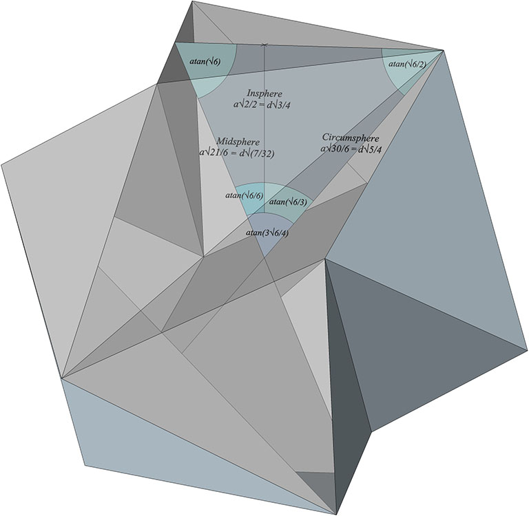
The Jessen’s circumsphere radius and the midsphere radius to its edge (a) forms a triangle of atan(√6), atan(√6/2), and atan(3√6/4). The insphere radius divides the latter angle into atan(√6/6) and atan(√6/3).
Insphere, midsphere, and circumsphere radii of the Jessen to its equilateral triangular face.
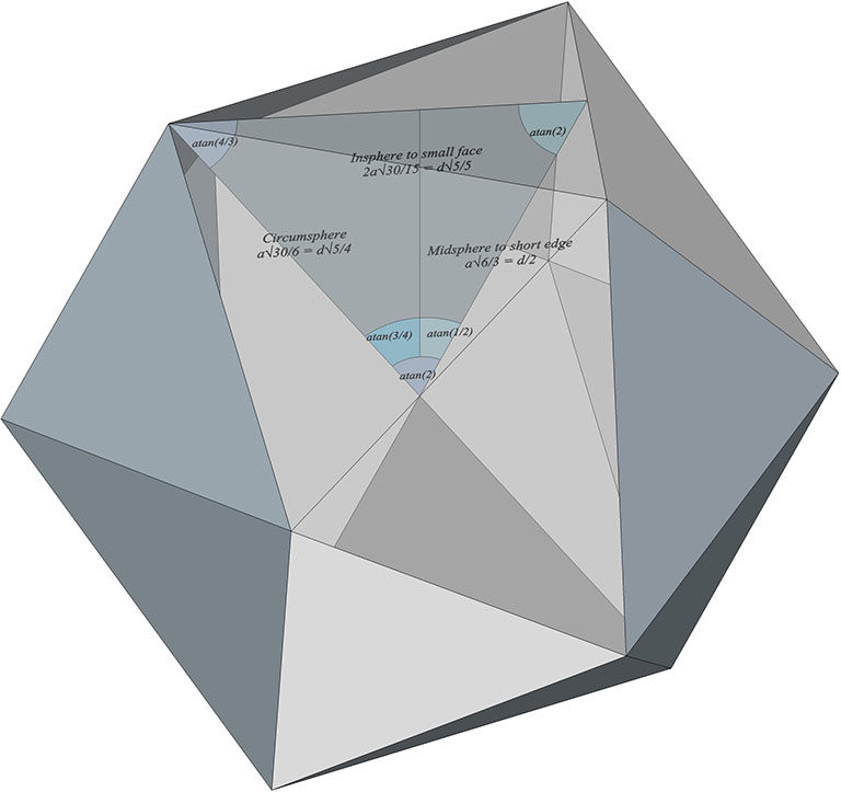
The Jessen’s circumsphere radius and the midsphere radius to its short (convex) edge (a’) forms an isosceles with rational trigonometry: atan(2), atan(4/3), and atan(2). The insphere radius divides the latter angle into atan(1/2) and atan(3/4).
Insphere, midsphere, and circumsphere radii of the Jessen to its isosceles triangle (convex) face.
The dimensions of the Jessen relative to its tendon (aka edge) length (a), and its strut (aka long edge) length (d) are provided below:
a = edge (tendon) length a’ = short edge length of convex face d = long edge (strut) length d = a × 2√6/3 a = d × √6/4 a’ = a × √6/3 = d × 1/2 Insphere radius = a × √2/2 = d × √3/4 Insphere radius to small face = a × 2√30/15 = d × √5/5 Midsphere radius = a × √21/6 = d × √14/8 Midsphere radius to short edge of convex face = a × √6/3 = d × 1/2 Midsphere radius to long edge of concave face = a × √6/6 = d × 1/4 Circumsphere radius = a × √30/6 = d × √5/4 Face angles (convex): atan(√5/2), atan(√5/2), atan(√5) Face angles (concave): atan(√2/2), atan(√2/2), acos(-1/3) Dihedral angles (convex form): acos(-3/5); acos(-√(3/5)) Dihedral angles: all 90° Cubic Volume (concave form) = a³ × 5√6/9 = d³ × 5/16 Tetrahedral Volume (concave form) = a³× 20√3/3 = d³ × 15√2/8 Cubic Volume (convex form) = a³ × 7√6/9 = d³ × 7/16 Tetrahedral Volume (convex form) = a³× 28√3/3 = d³ × 21√2/8
As noted earlier, the Jessen has rational cubic volume of 5/16 when the strut length (long edge) is of unit length; the Jessen has a rational tetrahedral volume of 7.5 when the strut length (long edge) preserves its length at vector equilibrium, i.e. √2. This is a gratifying result, and reinforces my view that the Jessen models an equilibrium phase of the isotropic vector matrix.
The Jessen icosahedron is a truncation of the pyritohedron.
Truncating the vertices of the pyritohedron (left) results in the convex form of the Jessen (right).
The struts (or long edges of the concave faces) of the Jessen align with the tetrakaidecahedra of the Weaire-Phelan matrix. (See: Tetrakaidecahedron and Pyritohedron.)
The struts of the 6-strut tensegrity align with the orthogonal distribution of tetrakaidecahedra in the Weaire-Phelan matrix.
These and other clues seem to point to a relationship between the tetrakaidecahedron-pyritohedron matrix (aka, the Weaire-Phelan structure) and tensor equilibrium, in addition to the relationship between the close packing of the voids in foam matrices with the close-packing of spheres and the distribution of nuclei in the isotropic vector matrix.
“The icosahedron positioned in the octahedron describes the S Quanta Modules. […] As skewed off the octa-icosa matrix, they are the volumetric counterpart of the A and B Quanta Modules as manifest in the nonnucleated icosahedron. They also correspond to the 1/120th tetrahedron of which the triacontahedron is composed.” —R. Buckminster Fuller, Synergetics, 988.110
The S quanta module is documented in Synergetics, but it doesn’t seem to have led Fuller anywhere. It was, I think, an attempt to rationalize the volume of the icosahedron, or, at the very least, to calculate the volume of the icosahedron that is inscribed inside the regular octahedron. See Icosahedron Inside Octahedron. Fuller’s operational method is provided here, along with my own calculations which, it should be noted, don’t always agree with Fuller’s.
With a regular icosahedron placed inside a regular octahedron with unit-length edges, the space not occupied by the icosahedron is subdivided into 24 irregular tetrahedron, 12 positive and 12 negative. These are the S quanta modules.
With a regular icosahedron placed inside a regular octahedron, the space not occupied by the icosahedron is subdivided into 24 irregular tetrahedra, 12 positive and 12 negative. These are the S Quanta Modules.
With the edge of the octahedron, a, taken as unity, the six edges of the S quanta module have the following lengths:
AC = a(3-√5)/2; CB = a/φ; AC+CB = a = 1 BA = a√(7-3√5); AD = a√(7-3√5)/2; BD = a√3×√(7-3√5)/2, and; CD = a√(7-3√5)/2
With the edge of the icosahedron, d, taken as unity, the six edges of the S quanta module have the following lengths:
AC = d√3/2 CB ≈ d×0.9045085 BA = d = 1 AD = d/2 BD = d√3/2 CD = d/2
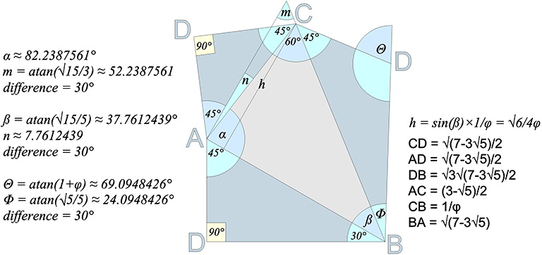
A (45°,α, 45°); B (30°, ß, Φ); C (45°,60°,45°), and; D (90°, 90°, (180°- Θ))
Note that the difference of 90° and α (i.e. 90°−82.2387561°) is 7.7612439°, or arctan(√(3/5))-30°. (See angle n in figure below.) This is the same angle that separates the icosahedron phases of the jitterbug.
The S quanta module unfolded from the external face (light gray triangle).
To calculate the volume of the S quanta module, we first find the area of its external face which will be taken as the S module’s base.
Base of external face of S module = BA = a√(7-3√5) = d 90° height of external face of S module = h = sin(ß) × BC = √6/4 × a/φ ≈ √6/4 × d×0.9045085 60° height of external face of S module = h’ = h × 2√3/3 = a√6/4φ × 2√3/3 = a√2/2φ ≈ √6/4 × d×0.9045085 × 2√3/3 ≈ √2d/2 × 0.9045085 Area of external face of S module (in equilateral triangles) = BA × h’ = a√(7-3√5) × a√2/2φ ≈ a² × 0.2063310 ≈ d × (√2d/2 × 0.9045085) 90° height of S module = AD 60° height of S module = h” = AD × √6/2 Volume of S module (in tetrahedra) = Area of external face × h”
The volume of the A quanta module is 1/24th that of the unit tetrahedron, or ≈ 0.041666, and the volume of the S quanta module is about 1.87415 times that of the A quanta module. Fuller thought the S module’s volume was 1.0820 times that of the A module’s. If we divide the volume of the S quanta module by 2, the volume of the A quanta module is about 1.06715 times that of the halved S quanta module, and that’s as close as I’ve come to Fuller’s figure, which remains a mystery.
The volume of space in the octahedron that is not occupied by the icosahedron is the S module’s volume times 24 ≈ 1.874147087. That leaves a volume of approximately 2.125852913 for the inscribed icosahedron. I haven’t found anything meaningful in these numbers.
Pyritohedra and tetrakaidecahedra close pack to constitute the Weaire-Phelan structure (or Weaire-Phelan “matrix” as I prefer to call it, and, when dimensioned appropriately, align precisely with the distribution of nuclei in the isotropic vector matrix. The unit vector (d in the illustration below) is identical with the unit vector (sphere diameter) of the isotropic vector matrix.
The pyritohedron (right) and the tetrakaidecahedron (left) combine to form the Weaire-Phelan structure (or matrix) and, when dimensioned appropriately, align with the distribution of unique nuclei (red) and shared nuclei (pink) in the isotropic vector matrix.
The pyritohedron and, presumably, the tetrakaidecahedron have identical rational volumes in both cubic and tetrahedral units of measure. For the cubic volume, we take the long edge of the pentagonal face as the unit length (a in the illustrations). For the tetrahedral volume, we take the diameter of the sphere as the unit length (d in the illustrations).
The dimensions of the pyritohedron’s pentagonal face are all related rationally to the length of its long edge, a, which is irrational with respect to d, the diameter of the unit sphere.
When we measure the angles, edge lengths, and radii of the pyritohedron, the numbers do not inspire confidence. It would seem unlikely that so many irrational numbers could possibly result in a rational, whole-number volume. But they do.
a = long edge or base of pentagonal face d = diameter of sphere* d = a × ³√4 × √2/2 a = d × ³(√2/2) = (d√2)/(³√4) = d√2 × ³√(1/4)
*d is identical with the unit vector of the isotropic vector matrix. In the Weaire-Phelan matrix, it aligns with the height vectors connecting the base with the peak of the smaller of the two pentagonal faces of the tetrakaidecahedron, and to the radial vectors connecting the height vector’s endpoints (see illustration below).
The unit vector, d, used in the volume calculations of the pyritohedron (right) is identical with the unit vector in the isotropic vector matrix, i.e. the diameter of the unit sphere. It aligns with the Weaire-Phelan matrix as the radial vectors and face heights in the tetrakaidecahedron (left).
The long edge of the pyritohedron’s pentagonal face, a, (which, when taken as unit length results in a cubic volume for the pyritohedron of 4a³) seems to be related to the diameter of the sphere, d, by ³(√2/2) or about 0.890898718. I don’t have a geometric proof to account for the appearance of this third root, but the number seems to work to at least 7 decimal places in my computer models, and the irrational roots cancel out perfectly in the volume calculations to produce the rational result of 24d³ for the tetrahedral volume.
*It should be possible to construct the pyritohedron from quanta modules, but may involve one or more variants of those quanta modules already described by by Fuller.
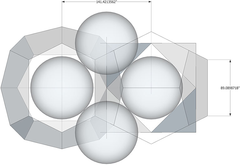
The image below shows my computer model with the calculated dimensions accurate to 7 decimal places.
If the circumsphere radius of the tetrakaidecahedron is of unit length (one sphere diameter), the long edge of the pyritohedron is, to an accuracy of at least seven decimal places, equal to √2׳√(1/4), or about 0.890898718, which produces a rational volume of 24 unit tetrahedra for both the pyritohedron and its complementary tetrakaidecahedron.
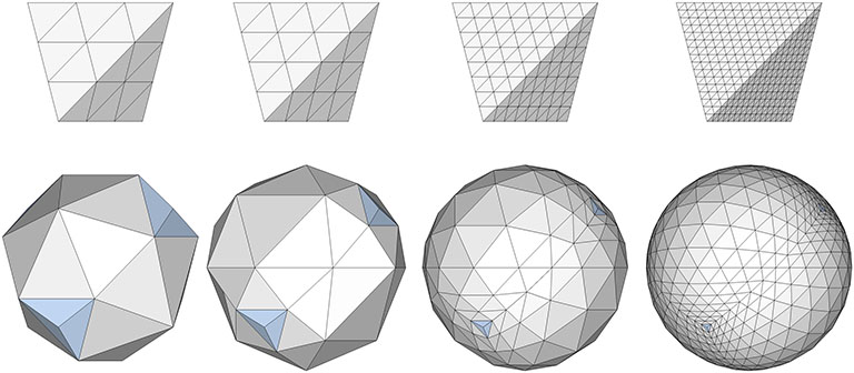
Geodesic polyhedra are convex polyhedra consisting of triangles, and include the spherical polyhedra generated by subdividing the faces of a tetrahedron, octahedron, or icosahedron into smaller triangles and projecting their crossings out to the underlying polyhedron’s circumsphere radius. Those based on the icosahedron are related to but not necessarily aligned with the 31 great circles of the icosahedron from which their name seems to have originated. The name “geodesic” refers to Fuller’s early conviction that only a triangular latticework of geodesic lines would serve to distribute local stresses evenly throughout the system he patented under the name “Geodesic Dome” in 1954. As the domes evolved into the systems of mostly partial great circles and lesser circles described here, the term “geodesic polyhedra” preserved the memory of that earlier conviction.
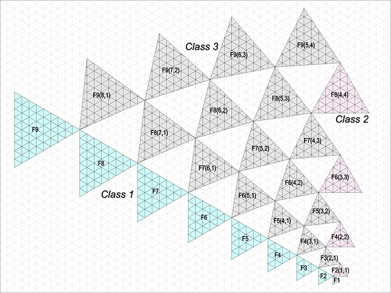
Geodesic polyhedra are defined by the equilateral triangles of the primary face (i.e., the face of the underlying tetrahedron, octahedron, or icosahedron) laid out on a 60° grid so that their vertices always align with grid crossings. This produces three classes of tiling or tessellation. The edges of the primary triangular face in Class 1 are parallel to the grid lines. The edges in Class 2 are perpendicular to the grid lines. Those in Class 3 are neither parallel nor perpendicular to the grid lines.
Geodesic polyhedra are divided into the three Classes defined by the orientation of the primary face laid out on a 60° grid. The edges of Class 1 polyhedra are parallel to the grid, Class 2 are perpendicular, and Class 3 skewed, neither parallel nor perpendicular to the grid.
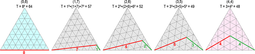
The frequency of each class is given by two numbers (b,c) representing the number of triangular modules along the grid lines connecting adjacent vertices. The general formula for the area, or the number of triangular modules that subdivide the primary face, is given by:
Area (T) = b² + c² + (b×c)
For Class 1, b is the edge length of the primary face; so, c is always 0 and the formula reduces to b². For Class 2, b = c, so the formula can be reduced to 3b².
The frequency of each Class of geodesic polyhedron is given by two numbers (shown in parentheses) representing the number of triangular subdivisions along grid lines connecting adjacent vertices (red and green lines). The primary face of the F8 polyhedra in Class 1 (blue), Class 3 (gray), and Class 2 (pink) are shown, along with their areas (T).
Class 1 Geodesics
Class 1 geodesics subdivide the primary face with lines parallel to the edges.
2F, 3F, 4F and 6F Class 1 geodesic polyhedra (icosahedron base)
Class 2 Geodesics
Class 2 geodesics subdivide the primary face with lines perpendicular to the edges.
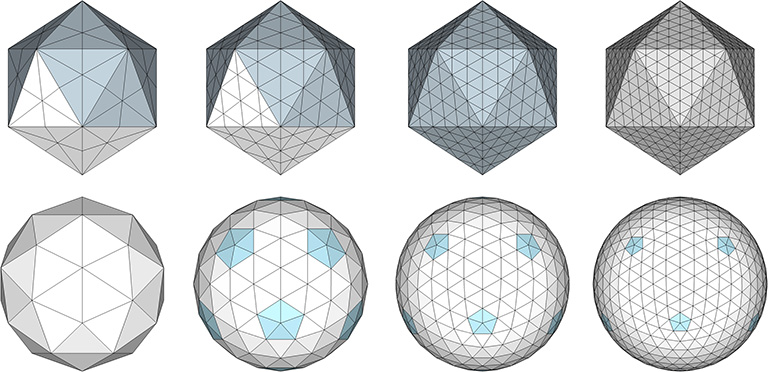
2F, 4F, 6F, and 8F Class 2 geodesic polyhedra (icosahedron base)
Class 3 Geodesics
Class 3 geodesics subdivide the face with lines that are askew to the edges, neither parallel no perpendicular.
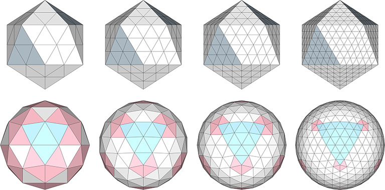
3F, 4F, 6F, and 8F Class 3 geodesic polyhedra (icosahedron base)
All of the geodesic polyhedra above have as their base the regular icosahedron. Being the most spherical, the icosahedron generates the most uniform tessellations. But the geodesic polyhedra may also be generated using the tetrahedron as their base, as in the following examples:
3F, 4F, 8F, and 16F Class 1 geodesic polyhedra (tetrahedron base)
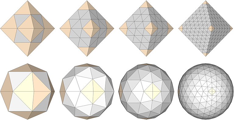
And they may also be generated using the octahedron as their base, as in these examples:
2F, 3F, 4F, and 8F Class 1 geodesic polyhedra (octahedron base)
The spherical tensegrities, whether based on the tetrahedron, octahedron, or icosahedron, have the shape of Goldberg polyhedra, the duals of geodesic polyhedra. Fuller held that all of his geodesic domes were, structurally, tensegrities. But then, any self-supporting structure can be described as a tensegrity. That is, all structural arrangements of vectors can be described as islands of compression in a continuous web of tension. Perhaps Fuller meant that his calculations were done on the spherical tensegrities, i.e., the tensor equilibrium phases of the tensegrity forms of the geodesic polyhedra. (See: Tensegrity, and; Tensegrity Equilibrium and Vector Equilibrium.) Many of Fuller’s domes do, in fact, have the appearance of Goldberg polyhedra. Fuller’s geodesic structures may be most accurately described as tensegrity composites incorporating both their spherical and polyhedron states.
The 2F Class 1 geodesic polyhedron as a Tensegrity composite, incorporating the 30-strut tensegrity sphere with its polyhedron counterpart, the tensegrity icosahedron.
An alternate construction of the 2F Class 1 geodesic polyhedron is achieved by reducing the the 120-strut tensegrity sphere to its polyhedron phase.
The 120-strut tensegrity sphere reduced to a 2F Class 1 geodesic polyhedron
Composite tensegrities, incorporating the spherical (Goldberg) and polyhedron (geodesic) phases of two or more frequencies may be possible without one interfering with the other. These may be easier to construct and would no doubt have incredible strength.
“You can “draw a line” only on the surface of some system. All systems divide Universe into insideness and outsideness. Systems are finite. Validity favors neither one side of the line nor the other. Every time we draw a line operationally upon a system, it returns upon itself. The line always divides a whole system’s unit area surface into two areas, each equally valid as unit areas. Operational geometry invalidates all bias.” —R. Buckminster Fuller, Synergetics, 811.04
All of Fuller’s geometry is “operational” in the sense that it is conveyed and verified by physical models. The operations of synergetics includes constructions of sticks and flexible connectors, quanta modules, struts and string, wire, elastic cord, paper disks, clusters of ping-pong balls, a list of materials and operations limited only by our imaginations. Science without models is like language without metaphor. In the absence of metaphor, language is merely encoded logic. And without models, Fuller argued, science is equally impoverished. We need metaphor to formulate and articulate as yet unidentified concepts, and models are the metaphors of science. (See: Model Making.)
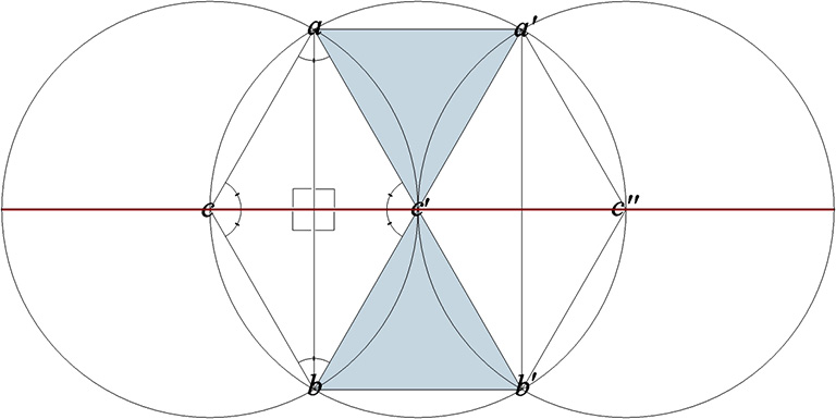
By way of introducing his operational geometry, Fuller would recall the basic operations of Euclidean geometry. Anyone who’s been through grade school has probably been taught how to use a draftsman’s compass, a straight edge, and a pencil, to repeat the familiar operation by which to find the perpendicular to a line and to construct an equilateral triangle.
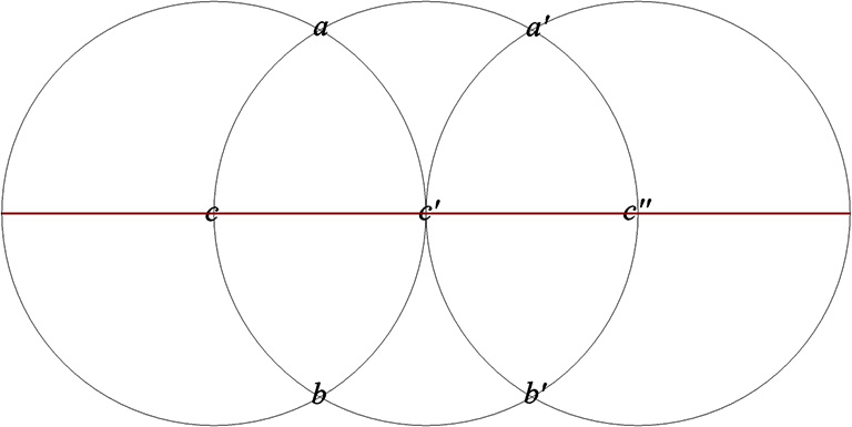
Begin by drawing a circle with the dividers of the compass tightened to a fixed radius. Next, with the straight edge, draw a line from its center (c) to the circle’s perimeter. Fix the compass on the point where the line crosses the circle’s perimeter (c’) and draw another circle. Repeat and draw a third circle centered at the point where the straight line crosses the perimeter of the second circle (c”).
Now you have three circles bisected by a straight line running through the the circle centers, c, c’, and c”. The second circle crosses the first at two points, a and b. The third circle crosses the second at two points, a’ and b’. Lines drawn from a to b, and from a’ to b’ are perpendicular to the line drawn between the circle centers. Finally, draw lines between adjacent points to create six equilateral triangles in the shape of a hexagon.
Fuller often argued that the key shortcoming of plane geometry is its failure to account for the surface on which its operations are performed. The surface is a tool, just like the dividers, the straight edge, and the stick we scratch the surface with.
With the surface in mind, Fuller re-imagined the above operations as follows:
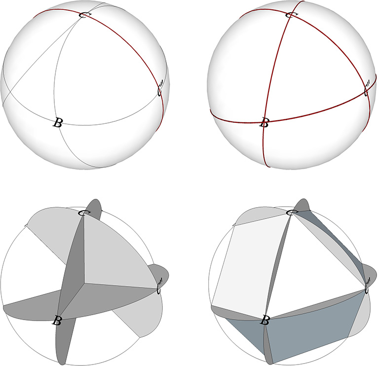
Begin by scribing a sphere. Granted, it isn’t possible to “scribe a sphere.” But we can imagine the process and perform the remaining operations on the surface of the sphere whose radius we are assured is identical with the fixed distance between the dividers of our compass. Mark a center anywhere on the sphere’s surface and draw a circle using the same compass. Next, just as before, draw a straight line from the center (C) to a point on the circle’s perimeter. And, remembering that straight lines on curved surfaces are, by definition, geodesics, we can continue drawing the line until it returns to the circle’s center and divides the sphere into two equal halves. Next, center the compass on one of the two points where the line crosses the perimeter of the circle and draw a second circle. Repeat, as above, to draw a third circle.
Now, when we connect the points as before with straight-line geodesics, we find that we have drawn four great circles. We know, operationally, that the length of the chords between the points is identical with the the sphere’s radius.
We have inadvertently constructed the eight equilateral triangles and six square faces of the vector equilibrium (VE). If we connect the points with the sphere center we create the eight tetrahedra and six half-octahedra that form the core of the isotropic vector matrix. And we have done it all operationally, without any calculations, and using only a compass, straight edge, and pencil.
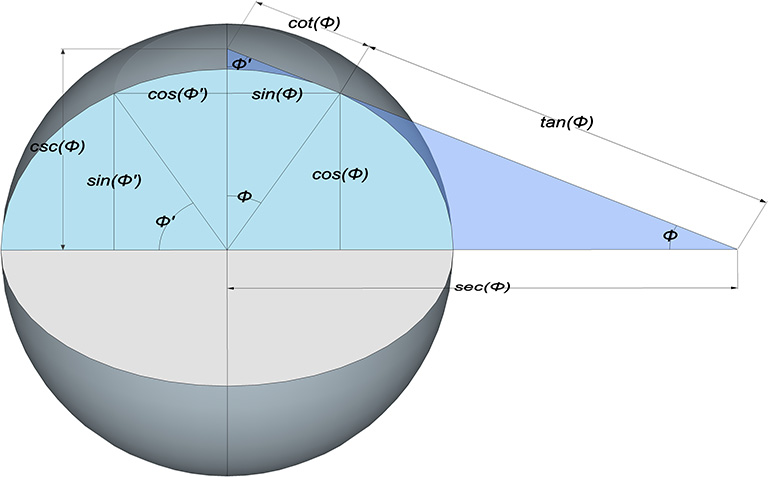
Fuller considered plane geometry to be a special case of the more general field of spherical trigonometry and topology. The Euclidean plane is a hemispheric section sliced through the middle of the sphere, and plane geometry is then the measurement of the chords whose central angles define the arcs of great circles drawn on the sphere’s surface.
All surfaces are curved. The flat surface in plane geometry is an abstraction, shown here as the hemispherical section of a sphere. Plane geometry is a special case of the more general spherical trigonometry and topology.
“… we observe the child taking the “me” ball and running around in space. There is nothing else of which to be aware; ergo, he is as yet unborn. Suddenly one “otherness” ball appears. Life begins. The two balls are mass-interattracted; they roll around on each other. A third ball appears and is mass-attracted; it rolls into the valley of the first two to form a triangle in which the three balls may involute-evolute. A fourth ball appears and is also mass-attracted; it rolls into the “nest” of the triangular group. . . and this stops all motion as the four balls become a self-stabilized system: the tetrahedron.“ —R. Buckminster Fuller, Synergetics, 100.331
“The mathematics involved in synergetics consists of topology combined with vectorial geometry. Synergetics derives from experientially invoked mathematics. Experientially invoked mathematics shows how we may measure and coordinate omnirationally, energetically, arithmetically, geometrically, chemically, volumetrically, crystallographically, vectorially, topologically, and energy-quantum-wise in terms of the tetrahedron.” —ibid., 201.01
Nature’s simplest structural system is the tetrahedron. Regular tetrahedra, however, do not combine to fill all-space (as do cubes, for example). In order to fill all-space, the regular tetrahedron must be complemented by the regular octahedron. Together they produce what Fuller conceived as the simplest, most powerful structural matrix in the universe, the octahedron-tetrahedron matrix, which he was able to patent in 1961 and subsequently copyright under the trademark name, the “octet truss.”
This complementary relationship between the tetrahedron and its space-filling counterpart, the octahedron, is demonstrated by stacking four tetrahedra vertex-to-vertex to create a larger tetrahedron. In doing so, we discover that we have inadvertently produced an octahedron at its center.
Stacking tetrahedra, vertex-to-vertex, to form a larger tetrahedron inadvertently produces an octahedron at its center. The two combine to fill all-space.
Fuller considered this system of all-space-filling tetrahedra and octahedra to be nature’s own coordinate system: the isotropic vector matrix.
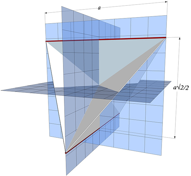
The regular tetrahedron is perhaps most easily conceived on the orthogonal grid as two unit length edges separated by a distance of √2/2 and oriented at 90° to the other (thick red lines in the figure below). Connecting their endpoints forms the the regular tetrahedron of edge length, a.
The regular tetrahedron constructed from coordinates on the orthogonal grid.
The Regular Tetrahedron
a = edge length
4 equilateral triangle faces, 4 vertices, 6 edges
Face angles all 60°
Central angles all arccos(-1/3) ≈ 109.4712°
Dihedral angle: atan(2√2) ≈ 70.5288°
Volume (in tetrahedra): a³
Cubic Volume: a³√2/12
A Quanta Modules: 24
B Quanta Modules: 0
Surface area (in equilateral triangles): 4a²
Surface area (in squares) 4a²√3/4
In-sphere radius (center to mid-face): a√6/12
Mid-sphere radius (center to mid-edge): a√2/4
Circumsphere radius (center to vertex): a√6/4
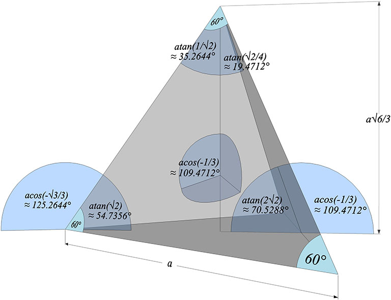
The surface, central, dihedral and other angles of the regular tetrahedron:
Surface, central, dihedral, and other angles of the regular tetrahedron
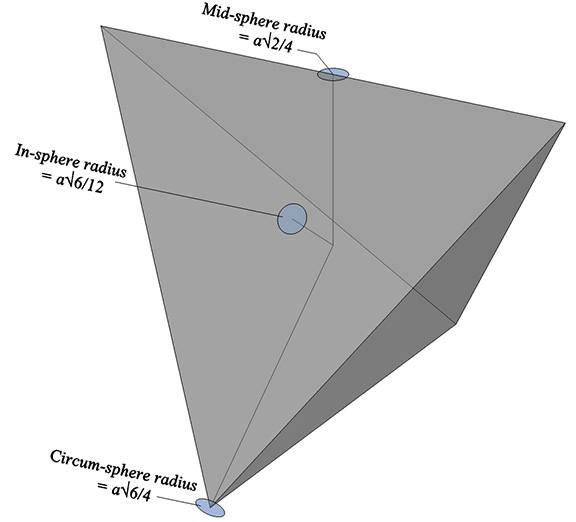
The in-sphere radius (center to mid-face), mid-sphere radius (center to mid-edge), and circumsphere radius (center to vertex) of the regular tetrahedron:
The in-sphere radius (a√6/2), mid-sphere radius (a√2/4), and circumsphere radius (a√6/4) of the regular tetrahedron
The regular tetrahedron has three natural poles, or axes, of spin, the three axes running between mid-edges.
The most natural pole, or axis of spin, of the regular tetrahedron runs from mid-edge to mid-edge.
The A quanta module is derived from the regular tetrahedron. Through symmetrical quartering and bisecting the regular tetrahedron is divided into 24 A quanta modules, 12 positive and 12 negative.
The regular tetrahedron defines and is constructed from 24 A Quanta Modules, 12 positive and 12 negative.
The regular tetrahedron can be constructed from a paper strip with three consecutive folds of arccos(-1/3), approximately 109.4712°.
The regular tetrahedron may be unfolded to, and refolded sequentially from, a single paper strip.
Spheres close pack as tetrahedra in even-numbered layers around octahedra (spaces) and VEs (spheres). In odd-numbered layers, the spheres surround a positive or negative tetrahedron (concave octahedron interstice). The growth pattern repeats every fourth layer, with the first layer surrounding a positive tetrahedron (concave octahedron interstice); the second layer surrounding an octahedron (concave VE space); the third layer surrounding a negative tetrahedron (concave octahedron interstice); and the fourth layer surrounding a VE (sphere).
Spheres close pack as tetrahedra in a pattern that repeats every four layers. Their relative position in the isotropic vector matrix is defined by what’s at their centers: a positive or negative tetrahedron (concave octahedron interstice); an octahedron (concave VE space); or VE (sphere).
Number of spheres in outer layer: 2F²+2 F = edge frequency, i.e., number of subdivisions per edge
Total number of spheres: [(N+1)³-(N+1)]/6 N = number of spheres per edge
A single sphere is free to rotate in any direction. Two tangent spheres are free to rotate in any direction but must do so cooperatively. Three spheres can rotate cooperatively about a single axis, i.e., they may involute and evolute along an axis perpendicular to the line connecting them with the center of the group. The addition of a fourth sphere acts as a lock, preventing all from rotating independently of the others. No rotation is possible, making the minimum stable closest-packed-sphere system: the tetrahedron.
Four spheres constitute the minimum self-stabilizing structural system, the tetrahedron.
Two triangular helical units combine to form one 4-sided tetrahedron. 1+1 = 4. Fuller would use this as a primary example of synergy and complementation. The two additional triangles were always there but invisible until the first two were combined into a system.
1+1=4. Two open triangles combine to form the four triangles of the tetrahedron.
The tetrahedron in its tensor-equilibrium phase has the overall shape of the Jessen orthogonal icosahedron. This 6-strut tensegrity is uniquely ambidextrous, i.e., neither right- nor left-handed; the vertex loops may be pulled inward to generate either a positive or a negative tetrahedron.
All structure is fundamentally reducible to tensegrity and this applies to the tetrahedron, show here transforming from its tensor-equilibrium phase into its polyhedral phase, alternating between positive and negative tetrahedra.
In the interstitial model of the isotropic vector matrix, the interstices occupy the positions defined by tetrahedra in the vector model, and by cubes in the quanta model. The interstices, i.e. the space between spheres close-packed as tetrahedra, describe a concave octahedron. (See Spheres and Spaces.)
Four spheres close-packed as tetrahedra disclose concave octahedra interstices at their common center.
This concave octahedron and its enclosing tetrahedron retain their shape and position throughout the jitterbug transformation. Only their orientation changes, with the tetrahedron rotating 90° between phases. See: The Jitterbug.
In any omni-triangulated structural system, that is, for any polyhedron structurally stabilized through triangulation:
the number of vertices (“crossings” or “points”) is always evenly divisible by two;
the number of faces (“areas” or “openings”) is always evenly divisible by four, and;
the number of edges (“lines,” “vectors,” or “trajectories”) is always evenly divisible by six.
This holds true for any polyhedron of whatever its size or complexity, just so long as its faces (areas, openings) are all triangulated and therefore constitute a “structure” by Fuller’s definition, i.e. any system that holds its shape without external support. The point here is that the same numbers, two, four, and six, fundamentally describe the tetrahedron:
The number of (non-polar) vertices in a tetrahedron is two;
The number of faces (“areas” or “openings”) in a tetrahedron is four, and;
The number of edges (“lines”, “vectors”, or “trajectories”) in a tetrahedron is six.
“When four tetrahedra of a given size are symmetrically intercombined by single bonding, each tetrahedron will have one of its four vertexes uncombined, and three combined with the six mutually combined vertexes symmetrically embracing to define an octahedron; while the four noncombined vertexes of the tetrahedra will define a tetrahedron twice the edge length of the four tetrahedra of given size; wherefore the resulting central space of the double-size tetrahedron is an octahedron. Together, these polyhedra comprise a common octahedron-tetrahedron system.” —R. Buckminster Fuller, Synergetics, 422.03
Nature’s simplest structural system is the tetrahedron. Regular tetrahedra, however, do not combine to fill all-space (as do cubes, for example). In order to fill all-space, the regular tetrahedron must be complemented by the regular octahedron. Together they produce what Fuller conceived as the simplest, most powerful structural system in the universe, the octahedron-tetrahedron system, which he was able to patent in 1961 and subsequently copyright under the trademark name, the “octet truss.”
If we stack six octahedra edge-to-edge to create a larger octahedron we discover that we have inadvertently produced eight tetrahedra at its center. The eight edge-bonded tetrahedra share a common vertex and form the vector equilibrium (VE).
Stacking octahedron, edge-to-edge to form a larger octahedron inadvertently produces eight tetrahedra at its center. The eight tetrahedra share a common center and form the VE.
Another name for this system of all-space-filling tetrahedra and octahedra is the isotropic vector matrix.
One of the simplest ways to construct the octahedron is to orient three squares to the three planes of the Cartesian grid, centered on the origin and turned so that each of their vertices lie on the axes.
The octahedron constructed from three equatorial squares intersecting symmetrically at 90°.
The surface, central, dihedral, and other interior and exterior angles of the regular octahedron.
Surface and interior angles of the regular octahedron
The in-sphere (center to mid-face), mid-sphere (center to mid-edge), and circumsphere (center to vertex) radii of the octahedron.
In-sphere, mid-sphere and circumsphere radii of the regular octahedron
The regular octahedron consists of 96 quanta modules, evenly distributed between A and B modules with 48 each.
Quanta module construction of the regular octahedron
The regular octahedron can be constructed from a single paper strip along seven consecutive folds of atan(2√2), or approximately 70.5288°, each. See also: Polyhedra From Polygonal Strips.
The regular octahedron can be constructed from a single paper strip with seven consecutive folds of atan(2√2).
The octahedron may be produced through the unfolding of one positive and one negative tetrahedron.
The octahedron produced by the unfolding of one positive and one negative tetrahedron.
The octahedron can also be produced from one positive or one negative tetrahedron alone. This produces an octahedron of four triangular facets and four empty triangular windows. This can be demonstrated through a kind of jitterbug transformation, as shown in the figure below.
Jitterbug-like oscillation between the regular tetrahedron and octahedron.
Spheres close-pack as octahedra around a central sphere or nucleus in even numbered layers only. The odd numbered layers surround a space, or concave vector equilibrium (VE).
Spheres close pack as octahedra around a central sphere in even-numbered layers. Odd-numbered layers surround a space (concave VE).
Number of spheres in outer shell: 4F²+2 F = edge frequency, i.e., the number of subdivisions per edge
Total number of spheres: (4N³+2N)/6 N = number of spheres per edge
The tensor equilibrium phase of the octahedron suggests the overall shape of the VE, with its six vertex loops forming the square “faces” of the VE. As with all polyhedra, with the exception of the tetrahedron (see: The Dual Nature of the Tetrahedron), the vertex loops are oriented in either a clockwise or a counter-clockwise direction and. when pulled in tight, form the six vertices of either the positive or the negative octahedron. (See also: 12-Strut Tensegrity Sphere and its Transformations.)
All structure is fundamentally reducible to tensegrity, and this includes the octahedron, shown here transforming between its tensor-equilibrium and polyhedral phases.
In the interstitial model of the isotropic vector matrix, the spaces between spheres occupy the positions defined by the octahedra in the vector model, and by one of the two rhombic dodecahedra in the quanta model. The spaces, i.e., the space between spheres close-packed as octahedra, describe a concave VE.
Six spheres close-packed as octahedra reveal a concave VE space at their common center.
All the structural (i.e. triangulated) polyhedra may be constructed from an even number triangular helices, or what Fuller called one half of a structural quantum. The tetrahedron and icosahedron require an equal number of clockwise and counter-clockwise helices. However, the octahedron is curiously constructed from an even number of clockwise, or an even number of counter-clockwise triangular helices, which seems to contradict our intuitive concept of structure as a knot of positive and negative forces.
This underscores, I think, our understanding of the octahedron as the space between the spheres, and the void between the tetrahedra, of the isotropic vector matrix.
The octahedron is constructed from an even number of clockwise or counter-clockwise triangular helices, unlike the tetrahedron and icosahedron which are constructed from an even number of both.
Note further that the endpoints of the helices converge on just two of the octahedron’s six vertices, resulting in a preferred axis of spin, and of wave propagation (see Isotropic Vector Matrix as Transverse Waves.)
All … regular, omnisymmetric, uniform-edged, -angled, and -faceted, as well as several semisymmetric, and all other asymmetric polyhedra other than the icosahedron and the pentagonal dodecahedron, are described repetitiously by compounding rational fraction elements of the tetrahedron and octahedron. These elements are known in synergetics as the A and B Quanta Modules. —R. Buckminster Fuller, Synergetics, Section 910.11
The pentagonal dodecahedron (or “regular” dodecahedron in conventional geometry) is the dual of the regular icosahedron; the 12 vertices of the regular icosahedron can be truncated to form the 12 faces of the pentagonal dodecahedron, and the 20 vertices of the pentagonal dodecahedron can be truncated to form the 20 faces of the regular icosahedron. (See: Icosahedron.)
But I think a more interesting symmetry is with the counterpart to the regular icosahedron that occurs in the jitterbug transformation of the isotropic vector matrix (see Icosahedron Phases of the Jitterbug). This counterpart to the regular icosahedron can be constructed from the pentagonal dodecahedron by truncating 8 of its 20 vertices along triangles formed by joining the vertex’s three face diagonals.
The space filling complement to the regular icosahedron (pink-white) constructed by truncations of the pentagonal dodecahedron.
Otherwise, the pentagonal dodecahedron does not appear in Fuller’s geometry. Like the icosahedron, it is incommensurate with the isotropic vector matrix and its volume is irrational whether measured in cubes or in tetrahedra.
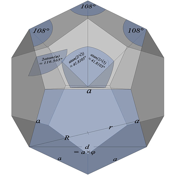
The pentagonal, or “regular,” dodecahedron with edge length, a, has the following dimensions when expressed in terms of the golden ratio (φ):
Volume (cubic, unit edge length (a): a³×5φ³/(5-√5)
Volume (tetrahedral, unit edge length (a): a³×φ³×30√2/(5-√5)
Volume (cubic, unit diagonal (d): d³×(φ+2)/2
Volume (tetrahedral, unit diagonal (d): d³×3√2(φ+2)
Quanta modules: n/a
Pentagonal Dodecahedron with edges (a), diagonals (d), in-radius (r), circum-radius (R), surface, central, and dihedral angles indicated.
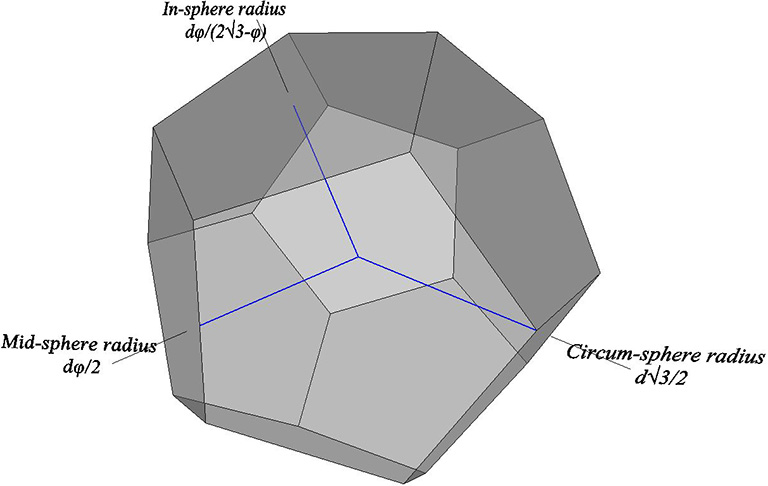
In-sphere, mid-sphere, and circumsphere radii of the pentagonal dodecahedron (φ = the golden ratio)
The volume of the pentagonal dodecahedron seems to be irrational regardless of which of its dimensions is taken as unity, and regardless of whether the volume is calculated in cubes or tetrahedra, as shown in the following table:
“Relationships Between First and Third Powers of F Correlated to Closest-Packed Triangular Number Progression and Closest-Packed Tetrahedral Number Progression, Modified Both Additively and Multiplicatively in Whole Rhythmically Occurring Increments of Zero, One, Two, Three, Four, Five, Six, Ten, and Twelve, All as Related to the Arithmetical and Geometrical Progressions, Respectively, of Triangularly and Tetrahedrally Closest-Packed Sphere Numbers and Their Successive Respective Volumetric Domains, All Correlated with the Respective Sphere Numbers and Overall Volumetric Domains of Progressively Embracing Concentric Shells of Vector Equilibria: Short Title: Concentric Sphere Shell Growth Rates.” —R. Buckminster Fuller, Synergetics, 971.01
The formulas for the close packing of spheres into clusters of triangles and tetrahedra follow the same sequential pattern as the number of unique pairings possible given a fixed number of objects. If N is the number of objects, the number of unique pairings is given by the formula, (N²-N)/2. The formula is the integral of the series (N-1)+(N-2)+(N-3)+…+(N-N), which represented graphically forms a triangle, with each element in the series forming a row of one less than the row below it. The formula for the total number of spheres comprising a triangle with n spheres along any one edge is (n²+n)/2. Because N in the previous formula equals n+1, we can rewrite the former as [(n+1)² – (n+1)]/2, and we can rewrite the latter as [(N-1)²-(N-1)]/2. In any case, if we stacked the results, they would form a tetrahedron. The formula for the total number of spheres comprising a tetrahedron with n spheres along any edge is [(n+1)³ + (n+1)]/6. This follows the pattern of the formula for the triangle, but the addition of ‘1’ follows the pattern of the formula for unique pairings.
Math sometimes hides rather than highlights patterns that would otherwise be obvious if we began with the geometric model. Spheres close pack as triangles and tetrahedra of frequency F, with F being the number of subdivisions of the edge vector. If we replaced n with F in the formulas for the close packing of spheres into triangles and tetrahedra, the formulas would be:
(F+2)²-(F+2)/2 = total spheres in triangle of frequency F (F+2)³-(F+2)/6 = total spheres in tetrahedron of frequency F.
Both follow the pattern of the formula for pairings, and the ‘+2’ is likely the same ‘+2’ we find in the sphere shell growth rate formulas:
2F²+2 = sphere shell growth rate tetrahedron; 4F²+2 = sphere shell growth rate of octahedron; 6F²+2 = sphere shell growth rate of cube;* 10F²+2 = sphere shell growth rate of VE; 12F²+2 = sphere shell growth rate of rhombic dodecahedron*.
*The shells of the cube and the rhombic dodecahedron are not close-packed.
Fuller attributes this “additive two” to the pole of spin, a property essential to the definition of any system. But when talking about an individual sphere, he attributes the “+2” to the sphere’s two surfaces—the convex exterior and the concave interior (see Anatomy of a Sphere). When F=0, the vector equilibrium (VE) consists of a single sphere, the nucleus. But the shell growth rate formula returns 10(0)²+2 = ‘2’. Fuller, however, does not discard this as a mathematical absurdity. The universe is finite, though unbounded, and the sphere, like all polyhedra, has both a concave inside, which contains a definite part of the finite universe, as well as convex outside, that contains an indefinite part of the finite universe. See The Multiplicative and Additive Two.
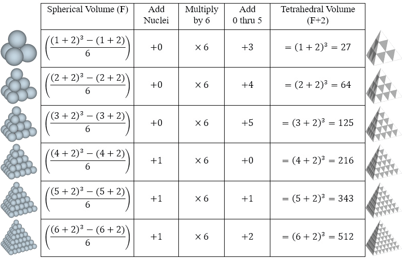
Fuller noticed a correlation between the tetrahedron’s spherical and tetrahedral volumes. By mathematically isolating the third power element in the formula for spheres, we observe a pattern that repeats in increments of 6, as disclosed in the following table:
By mathematically isolating the third-power element in the formula for the tetrahedron’s spherical volume, i.e. (F+2)³, we observe a six-part repeating pattern. Starting with with the spherical volume, and with each increase in frequency, F, we repeat the following steps: 1) Add the number of fully realized nuclei; 2) multiply by six, and then; 3) add the next number in the cycle 0, 1, 2, 3, 4, 5, 0, 1, 2, 3, etc. beginning with ‘3’ for F1.
Note further that the third-power element isolated from the spherical volume describes a tetrahedron with the same number of spaces as the number of spheres described by the original formula. For example, the spherical volume of the F1 tetrahedra in the left column of the above table is 4, and the number of spaces (i.e. octahedra) in the F2 tetrahedra in the right column is also 4. Remember that spheres and spaces exchange places in the oscillations of the isotropic vector matrix. (See also: Jitterbug, and Spheres and Spaces.)
I’m not convinced, however, that the first additive modifier (the second column of the table) is attributable to the number of nuclei. New nuclei emerge with every fourth layer, not every sixth, so Fuller may have either been mistaken, or he had a different understanding of what qualifies as a nucleus in tetrahedral clusters. Nor am I convinced of the significance that Fuller drew from the ratio between the 6 multiplier and the additive 0–5; The ratio of 6:5 is the same as 144:120, the volume of the spherical domain (there are 144 quanta modules in the rhombic dodecahedron), and the Basic Disequilibrium LCD Triangle (which divides the icosahedron by 120). Further, I do I see the 12:10 correlation that Fuller claimed existed between the volume of the outer shell in tetrahedra (see below), and the number of spheres in the outer layer of the VE (10F²+2). That’s not to say there isn’t one.
The formula for the tetrahedral volume of the VE is 20F³. We can isolate the shell volume by subtracting the volume of its interior VE, i.e., the VE of frequency (F-1): 20F³ – 20(F-1)³. The formula works out to be the following:
10(6F²-6F+2) = volume of outer shell (in tetrahedra) of VE of frequency F
which can be rewritten as: 10×[2+(12(F²-F)/2)].
Again, we have the same pattern, (F²-F)/2, seen in the formula for unique pairings. We also have the same ‘+2’ seen in the sphere shell growth rate formulas above. Further investigation would no doubt reveal other interesting patterns and correlations between the close packing of spheres and space-filling polyhedra.