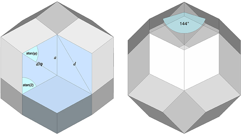
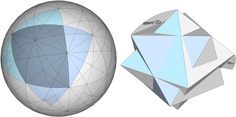
The rhombic triacontahedron has 30 faces, 60 edges, and 32 vertices. Each of its 30 faces is a golden rhombus, i.e., the length of its long diagonal is related to the length of its short diagonal by φ, the golden ratio: (√5+1)/2 ≈ 1.61803398875
If the long diagonal is taken as d, the length of its short diagonal is d/φ. Its face angles are atan(2) ≈ 63.434948823°, and 2atan(φ) ≈ 116.565051177°. Its dihedral angle is 144°.
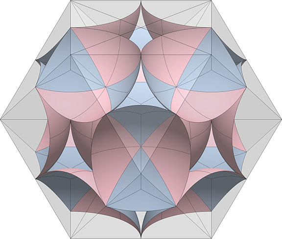
Surface angles (left) and dihedral angle (right) of the rhombic triacontahedron.
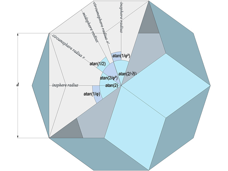
The central angle of its long diagonal, d, is atan(2) ≈ 63.434948823°. The central angle of its short diagonal, d/φ, is atan(2/√5) ≈ 41.810314896°. The central angle of its edge, a, is atan(2/φ²) ≈ 37.377368141°.
Central angles of the rhombic triacontahedron.
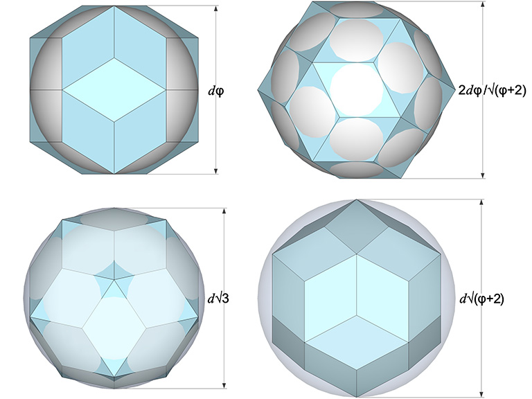
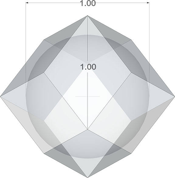
The in-sphere diameter is dφ. The mid-sphere diameter is 2dφ/√(φ+2). The circum-sphere diameter, i.e., the diameter measured by connecting opposite vertices bounded by four rhomboid faces, is d√(φ+2). The diameter measured by connecting opposite vertices bounded by three rhomboid faces, is d√3.
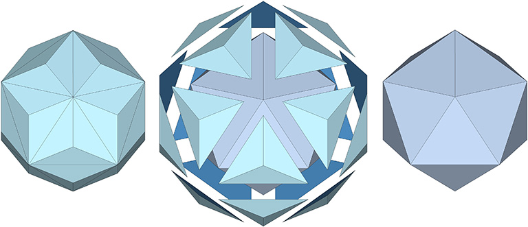
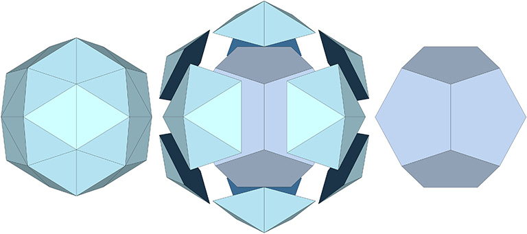
Truncating the rhombic triacontahedron on the long diagonal of its rhomboid face describes the regular icosahedron.
The regular icosahedron (right) is disclosed by truncating the rhombic triacontahedron (left) by the long diagonals that bisect its rhomboid face.
Truncating the rhombic triacontahedron on the short diagonal of its rhomboid face describes the pentagonal dodecahedron.
The pentagonal dodecahedron (right) is disclosed by truncating the rhombic dodecahedron (left) by the short diagonals that bisect its rhomboid face.
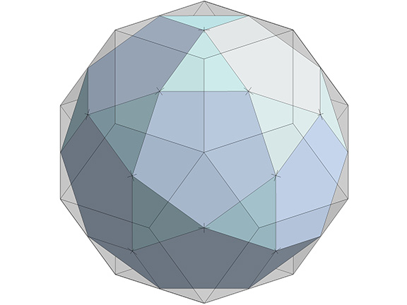
Connecting the face centers describes its dual, the icosidodecahedron.
The icosidodecahedron is disclosed by connecting the centers of the rhombic triacontahedron’s 30 rhomboid faces.
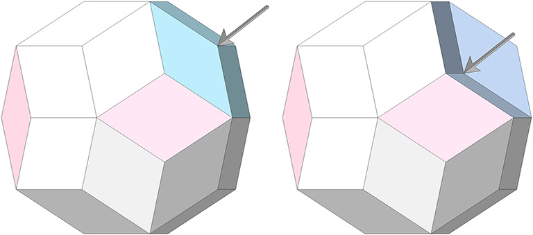
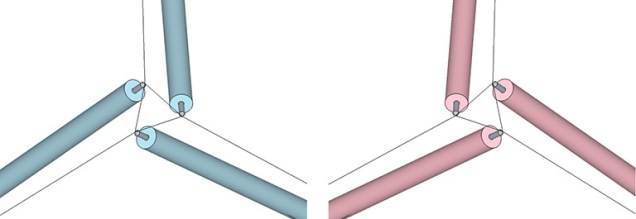
When a concentrated load is applied radially (toward the center) to any vertex of a polyhedral system, it tends to cause a dimpling effect. As the frequency or complexity of the system increases, the dimpling becomes progressively more localized, and proportionately less force is required to bring it about.
Applying radial pressure on a three-member vertex of the rhombic triacontahedron (left) results in a concave dimpling of its convex surface (right).
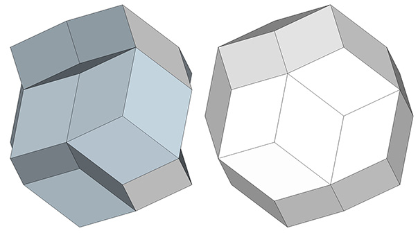
The rhombic triacontahedron may be a limit case in which the dimpling of its eight three-vector vertices produces a concave rhombic triacontahedron that close-packs with the convex triacontahedron to fill all-space.
The dimpled (or concave) rhombic triacontahedron will close-pack with the convex rhombic triacontahedron to fill all-space.
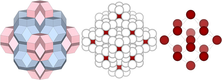
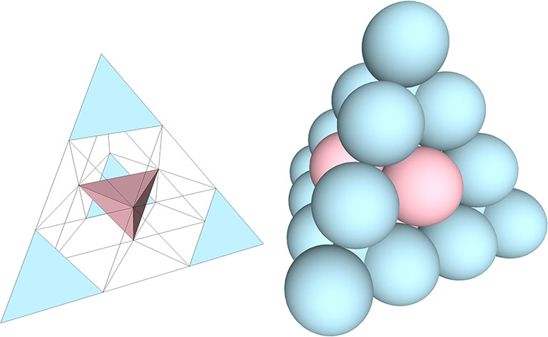
The convex and concave rhombic triacontahedra close-pack radially around a common center as rhombic dodecahedra, a pattern which is identical to the distribution of unique nuclei in the isotropic vector matrix. (See Formation and Distribution of Nuclei in Radial Close-Packing of Spheres.)
The concave and convex rhombic triacontahedra close-pack around a common center (left) in a pattern identical to the distribution of unique nuclei in the isotropic vector matrix. Nuclei isolated by their 12-sphere shells (center) define the 14 vertices of the rhombic dodecahedron (right).
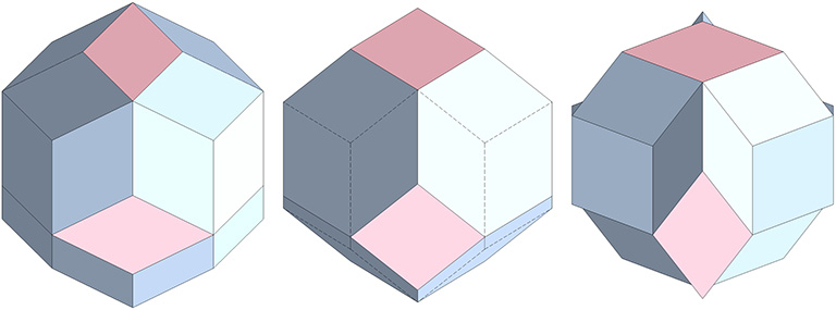
If the edge length is preserved, i.e., if we imagine the rhombic triacontahedron constructed of rigid struts and flexible connectors, it will undergo a jitterbug-like transformation into the all-space-filling Kelvin truncated octahedron at the halfway point in the transition between its convex and concave forms.
If the edge length is held constant, the rhombic triacontahedron (left) transforms into the all-space-filling Kelvin truncated octahedron (center) at the halfway point in the transition to its concave form (right).
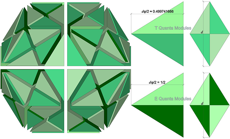
The in-sphere diameter of the rhombic triacontahedron with a tetrahedral volume of 5 is approximately 0.000517 less than the prime unit vector. This is an exquisitely small difference, and Fuller initially believed it to be due to the low resolution of the trigonometry tables he was using. The rhombic triacontahedron can be divided into 120 identical tetrahedra, and with a tetrahedral volume of five, each of the these 120 tetrahedra would have precisely the same volume as the A and B quanta modules, i.e., 1/24th of a unit tetrahedron. These he called the T quanta modules (‘T’ for ‘Triacontahedon’).
Subsequent calculations proved that the rhombic triacontahedron with a unit in-sphere diameter would have a tetrahedral volume of slightly more than 5. So, though his T quanta modules had a rational volume of 1/24th of the unit tetrahedron, the dimension corresponding to the in-sphere radius was awkward and irrational. The quanta module derived from the rhombic triacontahedron with a unit in-sphere diameter was subsequently named the E quanta module (‘E’ for ‘Einstein’). See T and E Quanta Modules.
The rhombic triacontahedron constructed of 120 T quanta modules has a tetrahedral volume of 5. The rhombic triacontahedron with a unit in-sphere diameter is constructed of 120 E quanta modules, and has a tetrahedral volume of slightly more than 5.
For a rhombic triacontahedron with a tetrahedral volume of 5:
120 T quanta modules
d = ³√(√2/6)
In-sphere diameter = dφ ≈ 0.999483332262
For a rhombic triacontahedron with an in-sphere diameter of 1:
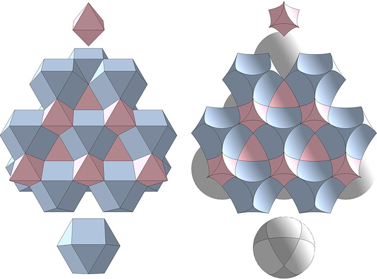
The tetrakaidecahedron of the Weaire-Phelan structure complements the pyritohedron to fill all-space. Together, they constitute what is presently determined to be the best solution to the Kelvin Problem: How can space be partitioned into cells of equal volume with the least area of surface between them?
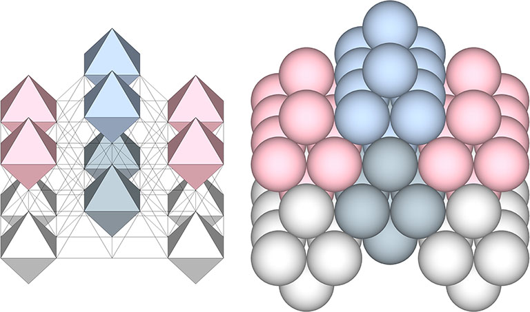
The pyritohedron (right) and the tetrakaidecahedron (left) combine to form the Weaire-Phelan structure (or matrix) and, when dimensioned appropriately, align with the distribution of unique nuclei (red) and shared nuclei (pink) in the isotropic vector matrix.
To summarize my conclusions:
If the sphere diameter, d, is taken as unity, the tetrahedral volumes of both the pyritohedron and the tetrakaidecahedron of the Weaire-Phelan structure work out to be precisely 24d³.
If its longest edge, a, is taken as unity, then d = 1/α, and the cubic volumes of both the pyritohedron and the tetrakaidecahedron of the Weaire-Phelan structure work out to be precisely 4a³.
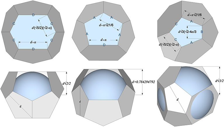
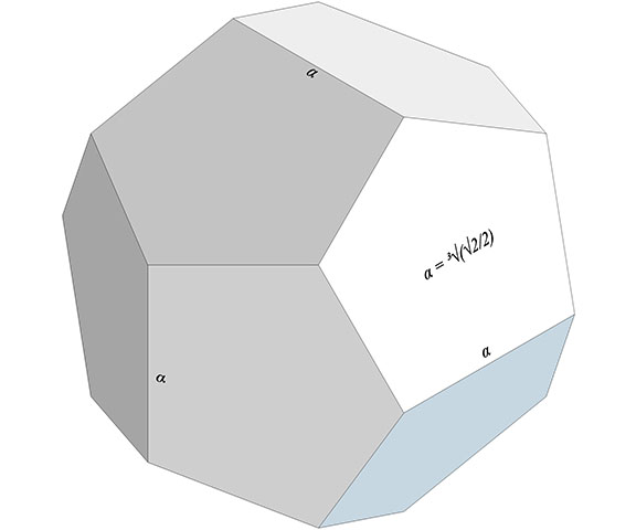
To satisfy the Kelvin problem, the volumes of the two shapes, i.e., the pyritohedron and its complementary tetrakaidecahedron, must be identical. This tetrakaidecahedron has three unique faces: two hexagonal faces; four large pentagonal faces; and eight smaller pentagonal faces, for a total of 14 faces — tetra (four), kai (+), deca (ten), hedron (face). To determine its volume, we’ll need the areas and in-sphere radii for each of its faces.
in-sphere radius to hexagonal face: d × √2/2
in-sphere radius to larger pentagonal face: d × ≈ 0.784294792 *
in-sphere radius to smaller pentagonal face: d × √3/2
* Though it should be possible to work out its precise value algebraically, I have so far been unsuccessful in resolving the in-sphere radius for the larger of the two pentagonal faces into whole number radicals and ratios.
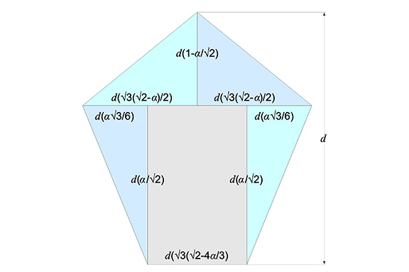
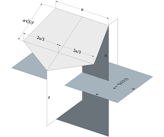
Edge lengths and insphere radii of the Weiare-Phelan structure’s tetrakaidecahdron. All measurements are in reference to the height, d, of the smaller pentagonal face, and the constant, α = ³√(√2/2), or the length of the long edge when d = 1.
In addition to the in-sphere radii as shown above, we must calculate the surface area for each of the faces. This is most easily accomplished by dividing each face into right triangles.
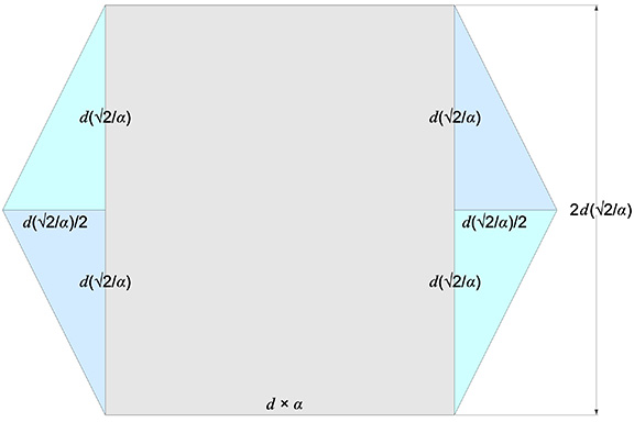
The hexagonal face is divided into four right triangles and one rectangle as follows:
Four right triangles of atan(1/2), with legs measuring d(√2/α) and d(√2/α)/2.
One rectangle measuring 2d(√2/α) by (d × α).
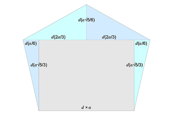
The larger of the two pentagonal faces is divided into four right triangles and one rectangle as follows:
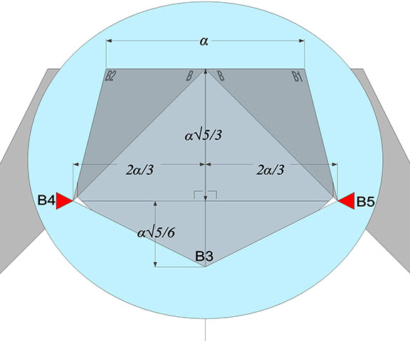
Two right triangles of atan(√5/4) with legs measuring d(α√5/6) and d(2α/3).
Two right triangles of atan(√5/10) with legs measuring d(α/6) and d(α√5/3).
One rectangle measuring d(α√5/3) by (d × α).
The smaller of the two pentagonal faces is divided into four right triangles and one rectangle as follows:
Two right triangles of atan(√6/3) with legs measuring d(α√5/6) and d(2α/3).
Two right triangles of atan(√6/6) with legs measuring d(α/√2) and d(α√3/6).
One rectangle measuring d√3(√2-4α/3) by d(α/√2).
If d is taken as unity (d = 1), then a = d × α = ³√(√2/2), and
The hexagonal face has a square area of ≈ 1.20629947402.
The cubic volume of its polyhedral cone is area/3 × √2/2 ≈ 0.28432751274
Multiplying by 2 (for the two hexagonal faces) ≈ 0.56865502548
Converting from cubic to tetrahedral units, multiply the above volume by 6√2 ≈ 4.825197896
Applying the same calculations to the large pentagonal faces, gives a total tetrahedral volume of 7.874010518.
And, applied to the small pentagonal faces, gives a total tetrahedral volume of 11.30079158.
4.825197896 + 7.874010518 + 11.30079158 = 24, and it therefore follows that its tetrahedral volume is 24d³.
If the long edge (the base of the larger pentagonal face) is taken as unity, the d in our equations = 1/α, then a = α/α = 1. The cubic volumes then are, respectively, 0.804199649, 1.312335086, and 1.883465264, and
0.804199649 + 1.312335086 + 1.883465264 = 4, and it therefore follows that its cubic volume is 4a³.
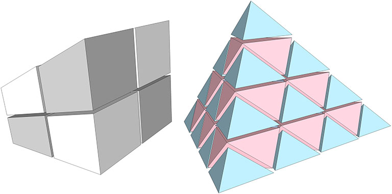
While irregular cubes subdivide into dissimilar six-sided polyhedra, any tetrahedron, regular or irregular, will always subdivide into similar tetrahedra and octahedra.
All tetrahedra, regular or irregular, subdivide into similar, equal-volume, tetrahedra and octahedron. This seems to be a property unique to the tetrahedron. An irregular cube, for example, subdivides into dissimilar parts.
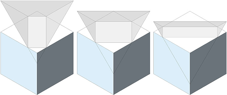
The perimeter of any rectangle defined by the section plane of a regular tetrahedron cutting perpendicularly through its edge-to-edge axis is a constant equal to 2 times its edge length.
As the tetrahedron is pulled out from the cube, the circumference around the tetrahedron remains equal when taken at the points where cube and tetrahedron edges cross.
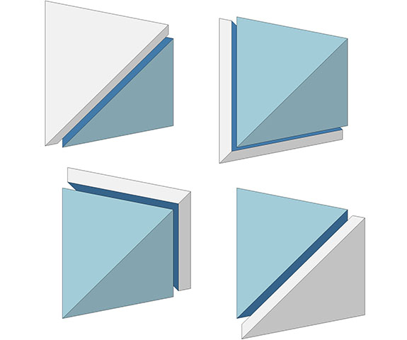
Any tetrahedron, regular or irregular, may be sliced parallel to any one or more of its faces without losing its basic symmetry. Or, as Fuller observed, “only the tetrahedron’s four-dimensional coordination can accommodate asymmetric aberrations without in any way disrupting the symmetrical integrity of the system.” (Synergetics, 100.304)
Any tetrahedron, regular or irregular, may be sliced parallel to any face without losing its basic symmetry.
The pulling outward or pushing inward of one or more faces of the tetrahedron accomplishes the same transformation as uniform scaling would achieve. This accommodation of asymmetrical aberrations while preserving its symmetrical integrity allows for the linear translation of the its center of gravity without actually moving the tetrahedron.
Pushing inward or pulling outward any face of the tetrahedron is identical with uniform scaling. But because it also changes its center of gravity, sequential pushing and pulling on different faces can effectively move the original tetrahedron to new coordinates.
The illustration below shows the same transformation, but with the two actions performed simultaneously, i.e., the pulling outward of one face occurs at the same time and at the same rate as the other face is pushed inward. This is essentially equivalent to a linear translation of the tetrahedron. We can accomplish any translation to any coordinates using this method, something that is possible with no other polyhedron.
The same transformation as above, but with the pushing and pulling happening simultaneously rather than sequentially, produces a transformation identical with positional translation without actually moving the tetrahedron.
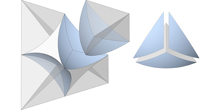
The tetrahedron may be turned inside out by pushing a vertex through the opening of its opposite face.
The tetrahedron is unique among the regular polyhedron in that it may be turned inside out by forcing any one of its vertices through the opening of its opposite face.
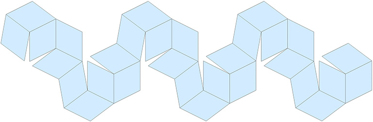
Each consecutive (non-oscillating) inside-outing produces a unique orientation of the tetrahedron, and results in an infinite or near-infinite number of helices or helical translations. See also: Tetrahelix.
Sequential inside-outing from a single tetrahedron at the center of this array produces an infinite or near infinite number of unique orientations of the tetrahedron.
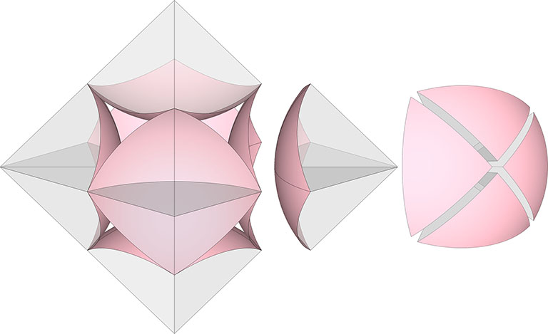
The tetrahedron may also turn itself inside-out by rotating three of its triangular faces outward from their common vertex like the petals of a flower. The process may be halted before the vertices rejoin on the opposite side, with the result being an octahedron rather than another tetrahedron. In the octet truss network, the octahedra occupy the spaces between tetrahedra. In the isostropic vector matrix, the octahedron defines the space between the spheres which in turn are defined by positive and negative tetrahedra sharing a common vertex at the center of the vector equilibrium (VE). It seems appropriate, therefore, to conceive of the octahedron as a positive and a negative tetrahedron turned inside-out, as the illustration below demonstrates.
A tetrahedron may be turned inside out by opening three of its faces like the petals of a flower. Two tetrahedra may be turned inside out to constitute the faces of the octahedron.
The tetrahedron is uniquely ambidextrous. By this, I mean that we can model the transformation from the positive to the negative tetrahedron non-destructively, i.e., without violating any of the principles that determine its structural or symmetrical integrity. To demonstrate, we need the tensegrity model.
As I’ve said elsewhere, anything in the universe (both physical and metaphysical as Fuller would insist on saying) that may be called structural is structured on tensegrity principles. The structural polyhedra (the tetrahedron, octahedron, icosahedron, and the geodesic polyhedra derived from them) can all be modeled as both polyhedral and spherical tensegrities. But only the tetrahedron may pass through its spherical phase and reverse polarity, with its vertices defined by either a clockwise or counter-clockwise tension loop. The remaining polyhedra are locked into a clockwise or counter-clockwise orientation, and cannot, non-destructively, reverse themselves. See also: Dual Nature of the Tetrahedron.
The vertices of all tensegrity polyhedra are structured in either a clockwise or a counter-clockwise orientation.
The transformation from a positive, or clockwise tetrahedron, to a negative, or counter-clockwise tetrahedron, is what spontaneously drives the jitterbugging of the isotropic vector matrix. See Jitterbug.
The tensegrity tetrahedron is unique among the the structural (tensegrity) polyhedra in that it may spontaneously transform between a clockwise and counter-clockwise orientation
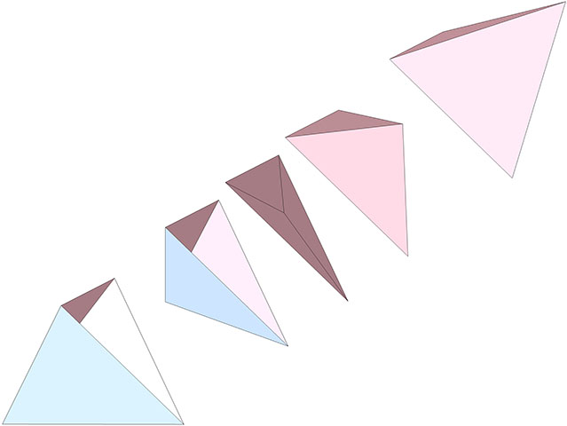
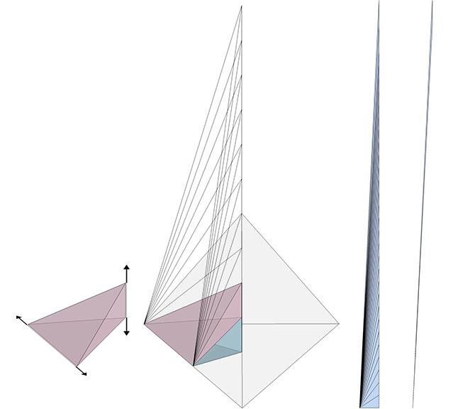
Fuller, taking his A and B quanta modules as inspiration, elaborated on their constancy of volume by continuing the progression out to infinity. Ultimately, we have something indistinguishable from a line, but with the volume of of the original tetrahedron. Fuller regarded this as a model of the photon. While we may imagine a photon traveling through space and time from its origin to its destination, the photon, from its own point of view, is already there.
The A (blue) and B (pink) quanta modules have equal volumes by virtue of equal base areas and identical altitudes. It follows that a line, originating at the center of the triangular base of a regular tetrahedron, projected through the apex of the tetrahedron and subdivided into equal increments, will produce additional modules with the same volume as the original A or B Module. As the incremental line approaches infinity the modules will tend to become lines (for right), but lines still having the same volume as the original A or B modules.
A similar constancy is observed when we orient the tetrahedron on its edge-to-edge axes. The highly skewed half-octahedra in the illustration below each have the same volume as the original tetrahedron.
Half-octahedra produced by pulling one of edges vertically away from its opposing edge, along with one of its faces, in increments equal to its mid-sphere (edge-to-edge) diameter will have the same volume as the original tetrahedron.
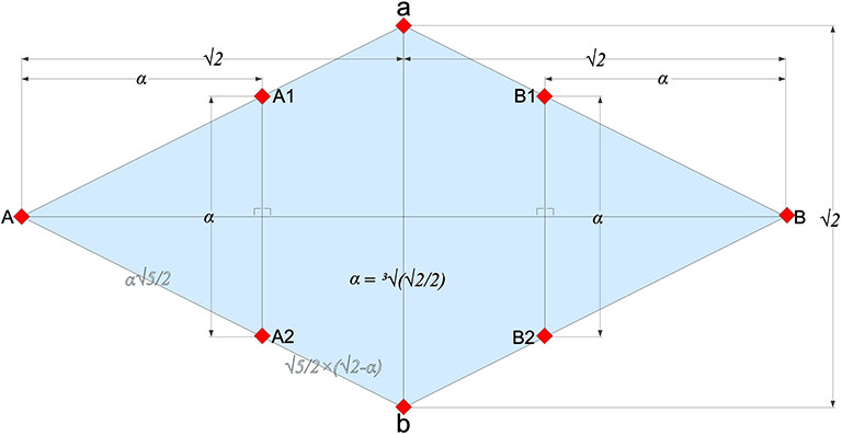
Begin with a 2√2 by √2 rhombus. Mark the vertices of the long diagonal A and B, and the vertices of the short diagonal a and b. On AB, mark points ³√(√2/2), about 0.8908987, in from each end. Lines perpendicular to AB and passing through these points bisect the edges of the rhombus at A1, A2, B1, and B2. (See illustration.)
The first step in this construction of the Weaire-Phelan tetrakaidecahedon is a 1×2 rhombus dimensioned and scribed as indicated. The points A1, a, B1, B2, b, and A2 define one of its two hexagonal faces.
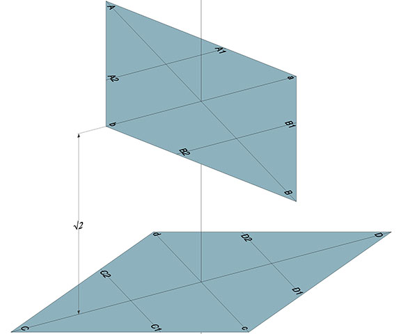
Replicate the rhombus, rotate 90°, and separate (along the center face normal vector) by √2. Mark points as above, substituting C c for A a, and D d for B b.
A second rhombus spaced one unit (√2) from the first and rotated 90° defines the vertices of the 2nd hexagonal face of the tetrakaidecahedron: C2, d, D2, D1, c, and D2.
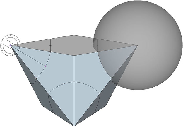
Connect the vertices to and create faces: BCcB; BDcB; bCBb; aDBa; ACdA; ADdA; aDAa, and; bCAa. Measure the distance, r, from A to either A1 or A2, and, using this length as the radius, scribe arcs from A on each of its adjacent faces. Repeat for B, C, and D.
The precise value of r is ³√(√2/2)×√5/2, or about 0.996055.
A ten-sided polyhedron is constructed by connecting the vertices of the two rhombuses. Arcs scribed onto the faces from each of its four acute corners will be used to define the planes of its four large pentagonal faces.
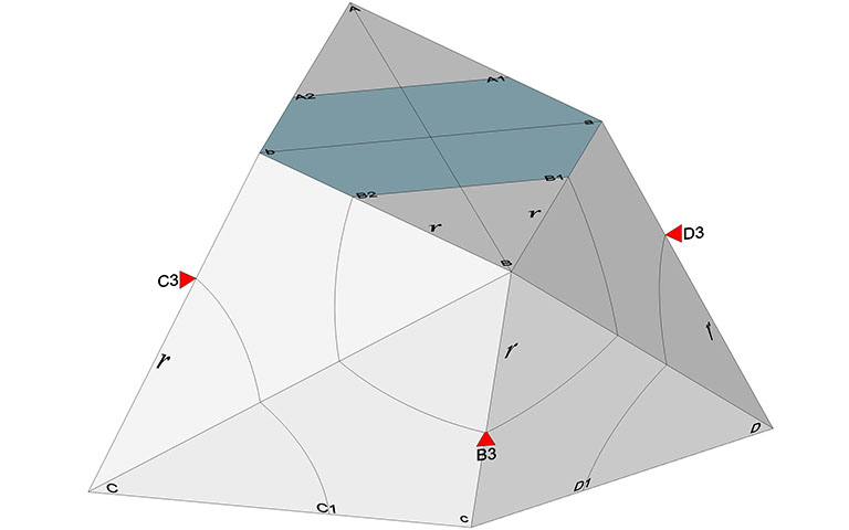
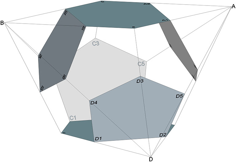
The scribed arcs locate the peaks of the tetrakaidecahedron’s four larger pentagonal faces at A3, B3, C3 and D3 (see illustration).
The scribed arcs locate the peaks of the larger of the two pentagonal faces, indicated here by red triangles B3, C3, D3, and A3 (hidden).
Each of the tetrakaidecahedron’s four larger pentagonal faces occupy a plane defined by the three vertices identified so far. At corner B, the plane (the blue disk in the illustration below) is defined by B1, B2, and B3. To locate the remaining two vertices, draw a line from the midpoint between B1–B2 to B3, and mark a point on this line ³√(√2/2)×√5/3 from the midpoint, or ³√(√2/2)×√5/6 from B3. A perpendicular through this point parallel to B1–B2 intersects BC and BD at B4 and B5, completing the pentagonal face (see illustration).
The three points identified so far from corner B (B1, B2, and B3) define the plane (blue disk) occupied by the pentagonal face. This enables us to determine the positions of the pentagon’s remaining two vertices, B4 and B5. Note these points are not identical with the intersections of the arcs we scribed earlier, which lie slightly above the plane.
Repeating the steps for each corner A, B, C and D, produces four pentagonal faces in addition to the two hexagonal faces defined in the first step.
The tetrakaidecahedron with its two hexagonal faces (top and bottom), and its four, larger pentagonal faces as constructed with the operations described.
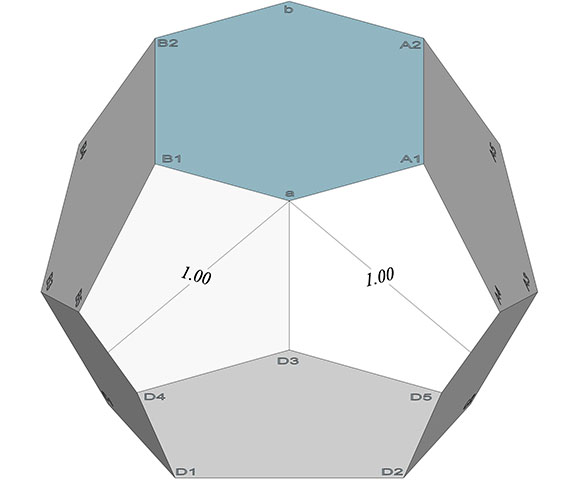
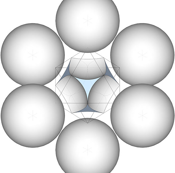
The points surrounding the remaining empty space should all lie on the same plane and define the eight smaller pentagonal faces of the Weaire-Phelan tetrakaidecahedron. A line bisecting their faces from the peak to mid-base should be of unit length, or, in terms of the isotropic vector matrix, one sphere diameter.
The Weaire-Phelan tetrakaidecahedron. The height of its eight smaller pentagonal faces is identical with the diameter of the radially close-packed spheres that define the isotropic vector matrix.
Pyritohedron
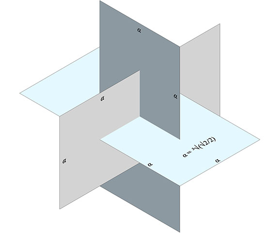
Begin with three, intersecting and mutually perpendicular 1 x 2 rectangles all sharing a common center. To construct a pyritohedron that will complement the Weaire-Phelan tetrakaidecahedron to fill all-space, the rectangle’s short edge will be ³√(√2/2) and the long edge will be twice that length (see illustration).
The first step in the creation of the pyritohedon is to construct three mutually perpendicular 1×2 rectangles. The length of the short edge, α, is ³√(√2/2) and the long edge is 2×α.
The twelve pentagonal faces of the pyritohedron are identical with the four larger pentagonal faces of the tetrakaidecahedron, and they are constructed using a method nearly identical with the procedure for the four larger pentagonal faces of the tetrakaidecahedron described above. Each face plane is defined by the the short edge of one rectangle, and the nearest corners of the rectangle perpendicular to that edge.
The twelve faces of the pyritohedron are constructed similarly to the larger of the pentagonal faces of the tetrakaidecahedron. The plane of each is defined the ends of the short edge of one rectangle and the nearest corners of the rectangle perpendicular to that edge.
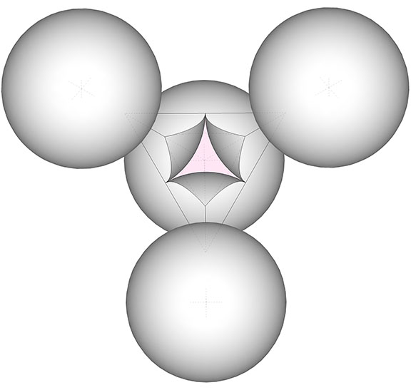
This pyritohedron has a rational volume of 24d³ in unit tetrahedra, where d is is the diameter of the unit sphere in the isotropic vector matrix or the height of the tetrakaidecahedron’s smaller pentagonal face. Its cubic volume of 4α³, where α is the length of the pyritohedron’s long edge. This volume should be identical with that of its companion tetrakaidecahedron. See Pyritohedron Dimensions and Whole-Number Volume, and Tetrakaidecahedron Dimensions and Whole Number Volume.
The pyritohedron. With the long edge equal to ³√(√2/2), it complements the Weaire-Phelan tetrakaidecahedron to fill all-space, and isolates the the nuclear domains of the radially-close-packed unit spheres of the isotropic vector matrix.
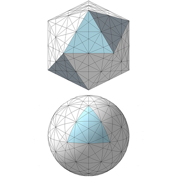
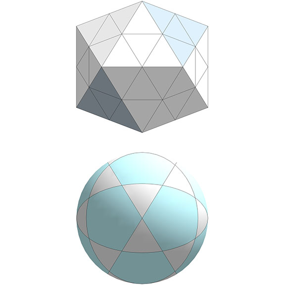
The figure below illustrates the full set of 31 great circles described by rotations about the regular icosahedron’s axes of symmetry.
The 31 great circles of the icosahedron as projected onto the planar icosahedron (top) and sphere (bottom).
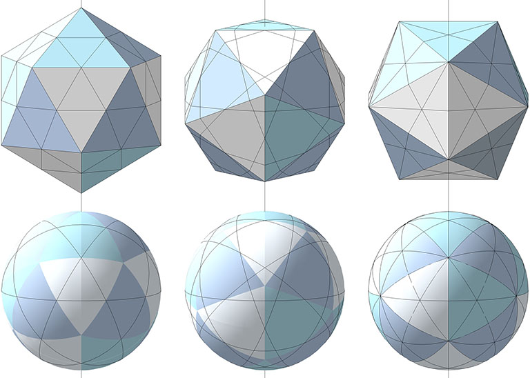
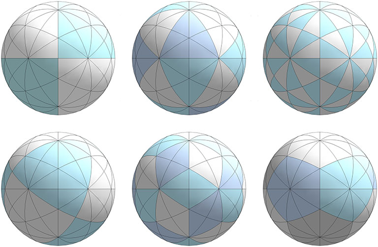
The 31 great circles are divided into three sets according to their spin axes. Axes running through diametrically opposing vertices generate the set of 6 great circles. Axes running through opposite faces generate the set of 10 great circles. And axes running through the midpoints of diametrically opposing edges generate the set of 15 great circles.
Left to right: the set of 6 great circles on axes running though opposing vertices; the set of 10 great circles on axes running through the centers opposing faces, and; the set of 15 great circles on axes running though he midpoints of opposing edges.
6 Great Circles
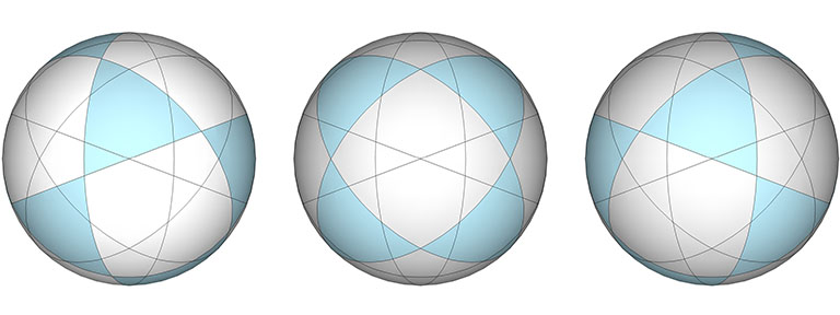
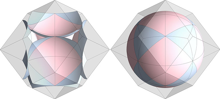
The set of 6 great circles circumscribes the equators of the six spin axes that pass through the icosahedron’s opposing vertices, and together they disclose the spherical icosidodecahedron.
The set of 6 great circles of the icosahedron disclose the spherical icosidodecahedron.
15 Great Circles
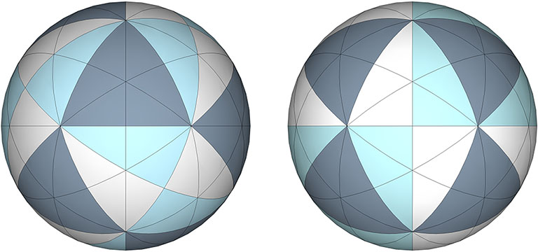
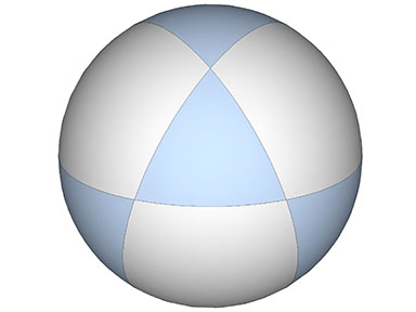
The set of 15 great circles disclose the two orientations of the spherical octahedron, the spherical icosahedron, pentagonal dodecahedron, rhombic triacontahedron, and the 120 basic disequilibrium LCD triangles.
The set of 15 great circles of the icosahedron disclose two orientations of the spherical octahedron (left); the spherical icosahedron (top middle); the rhombic triacontahedron (bottom middle); the 120 basic disequilibrium LCD triangles (top right); and the pentagonal dodecahedron (bottom right).
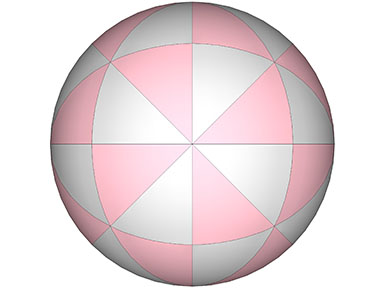
The same spherical icosahedron is symmetrically aligned with both orientations of the spherical octahedron. See also: Icosahedron Inside Octahedron.
Both orientations of the spherical octahedron align symmetrically with the same spherical icosahedron disclosed by the 15 great circles of the icosahedron.
10 Great Circles
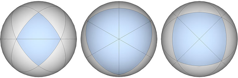
The set of 10 great circles discloses three orientations of the spherical vector equilibrium (VE).
Three orientations of the vector equilibrium (VE) as disclosed by the 10 great circles of the icosahedron.
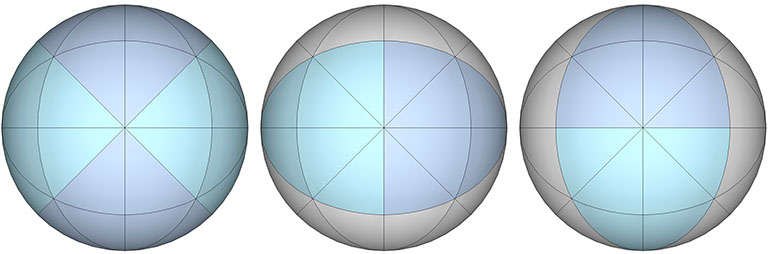
The same spherical icosidodecahedron (generated from the six great circles) is symmetrically aligned with all orientations of the spherical vector equilibrium (VE).
All three orientations of the VE as disclosed by the 10 great circles of the icosahedron are symmetrically aligned with the same icosidodecahedron disclosed by the 6 great circles.
The figure below illustrates the full set of great circles in the context of the vector equilibrium (VE), both the planar VE (top), and spherical VE (bottom). Note that twelve great circles converge, cross, or are deflected at each of the twelve vertices, and at the centers of each triangular face.
The 25 great circles of the vector equilibrium (VE)
The 25 great circles are divided into four sets according to their spin axes. Axes running through opposite square faces generate the set of 3 great circles. Axes running through the centers of opposite triangular faces generate the set of 4 great circles. Axes running through diametrically opposing vertices generate the set of 6 great circles. And axes running through the midpoints of diametrically opposing edges generate the set of 12 great circles.
Left to right: Set of 3 great circles on axes through opposing square faces; Set of 4 great circles on axes running through opposing triangular faces; Set of 6 great circles on axes running through opposing vertices; Set of 12 great circles with axes running through opposing edges.
3 Great Circles
The set of 3 great circles discloses the spherical octahedron.
The spherical octahedron disclosed from the set 3 great circles, with one face highlighted.
4 Great Circles
The set of 4 great circles discloses the spherical vector equilibrium (VE).
The spherical VE disclosed from the set of 4 great circles, with its triangular faces highlighted.
6 Great Circles
The six great circles disclose the spherical rhombic dodecahedron, the spherical tetrahedron (both positive and negative), and the spherical cube.
The set of 6 great circles disclosing, left to right: the spherical rhombic dodecahedron; the spherical tetrahedron, and; the spherical cube, each with one face highlighted.
The six great circles complement the three great circles to disclose three additional octahedra.
The sets of 3 and 6 great circles disclose three additional spherical octahedron.
The sets of 3 and 6 great circles of the VE disclose the 48 basic equilibrium LCD triangles.
12 Great Circles
The twelve great circles of VE do not appear to disclose, by themselves, any of the regular polyhedra. However, in combination with the 4 and 6 great circle sets, the 12 great circles do disclose an alternate spherical regular octahedron that is curiously askew from the others, rotated 30° on the z axis, and atan(√2) on the y axis.
The 4, 6, and 12 great circles of the VE each contribute one edge to disclose a spherical octahedron whose axes are curiously skewed from all the other polyhedra the 25 great circles of the VE disclose.
“The closest-packed symmetry of uniradius spheres is the mathematical limit case that inadvertently captures all the previously unidentifiable otherness of Universe whose inscrutability we call space. The closest-packed symmetry of uniradius spheres permits the symmetrically discrete differentiation into the individually isolated domains as sensorially comprehensible concave octahedra and concave vector equilibria, which exactly and complementingly intersperse eternally the convex “individualizable phase” of comprehensibility as closest-packed spheres and their exact, individually proportioned, concave-in-betweenness domains as both closest packed around a nuclear uniradius sphere or as closest packed around a nucleus-free prime volume domain.” —R. Buckminster Fuller, Synergetics, 1006.12
Spaces, like spheres, have surfaces. The interstitial model of the isotropic vector matrix (IVM) makes evident that it is the sphere’s surfaces (both its convex and its concave surfaces) that matter. Electric charge is carried on the surface of the conductor. Molecular biology is all about the lock and key system of protein surfaces and shapes. The surface of the “space” in the isotropic vector matrix is a continuity broken only be the seams at the interface of the concave “spaces” and “interstices” (see below). These seams align with the four great circles of the vector equilibrium (VE), and describe the most efficient paths between the points of contact with adjacent spheres. See also: Anatomy of a Sphere.
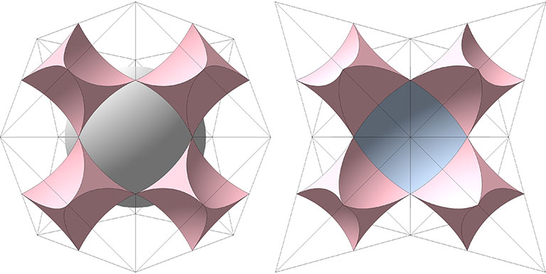
The figure below shows the exact correlation between two models of the isotropic vector matrix, a correspondence that Fuller attempted to describe in the excerpt I’ve quoted above.
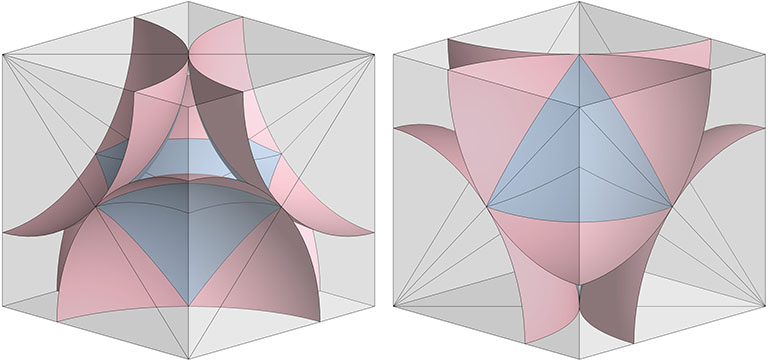
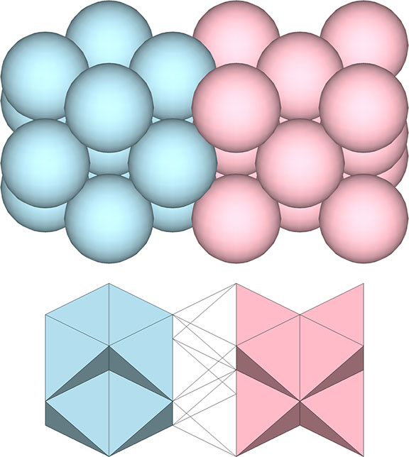
Space Filling of Octahedron and Vector Equilibrium: The packing of concave octahedra, concave vector equilibria, and spherical vector equilibria corresponds exactly to the space filling of planar octahedra and planar vector equilibria. Exactly half of the planar vector equilibria become convex; the other half and all of the planar octahedra become concave.
Though the VEs (blue) and octahedra (pink) on the left align with the spaces (blue) and interstices (pink) on the right, close inspection of the above models reveals a key difference. The model on the left does not distinguish between spheres and spaces. While on the right the difference is obvious, on the left both spheres and spaces are represented by identical VEs. The ambiguity is apt: In the isotropic vector matrix, there is a one-to-one identity between the spheres and spaces; one is simply the other turned inside out.
The model on the right is what I’m calling the interstitial model of the isotropic vector matrix. It consists of concave vector equilibrium (VE) spaces and concave octahedron interstices. The concave VE is the shape of the void at the center of six close-packed spheres defining the octahedron. The concave octahedron is the shape of the void at the center of four close-packed spheres defining the tetrahedron.
Concave VE (“space”)
Because it occupies the space in the isotropic vector matrix that is replaced by a sphere in the jitterbug transformation, I reserve the term “space” for the concave VE at the common center of the six close-packed spheres of the regular octahedron.
The void at the center of the six close-packed spheres centered on the vertices of the regular octahedron has the shape of a concave vector equilibrium (VE). In the jitterbug transformation, this “space” is turned inside-out to define the spherical VE or “sphere.”
Concave Octahedron (“interstice”)
The void at the center of four close-packed spheres has the shape of a concave octahedron which I call the “interstice” to distinguish it from the “space” referred to above. The interstices maintain both their shape and position during the jitterbug transformation, while their 90° rotations articulate the sphere-to-space oscillations described below.
The void at the center of the four spheres centered on the vertices of the regular tetrahedron has the shape of a concave octahedron. These “interstices” are rotated 90° to alternately define the spheres and spaces that exchange places in the jitterbug transformation.
Spherical Domains
The polyhedra of the isotropic vector matrix divide the spheres into rational sections which, when added together, constitute the polyhedron’s spherical domain. Fuller thought this rationality was sufficient to eliminate pi (π) from his geometry. He’d already shown that the volumes of most polyhedra were rational if instead of the cube we used the regular tetrahedron as the unit volume. And if we replaced the irrational volume of the sphere with the rational sections carved from the rational polyhedra, pi was irrelevant.
Rhombic Dodecahedron
144 quanta modules
1 spherical domain
Vector Equilibrium (VE)
480 quanta modules
3.40 spherical domains
Cube
72 quanta modules
1/2 spherical domain
Octahedron
96 quanta modules
3/5 spherical domain
Tetrahedron
24 quanta modules
1/5 spherical domain
Octahedron
The six spheres at the vertices of the octahedron define the concave vector equilibrium space at its center. The planar facets of each vertex carve a 1/10 section from its sphere. The 1/10 section is further subdivided to form the four 1/40 sections used in the spherical domain calculations. The total spherical domain of the planar octahedron is 3/5.
The planar octahedron cuts 1/10 sections from each of its six spheres, for a total spherical domain of 3/5. Each of these 1/10 sections is further subdivided into four 1/40 sections which are used to calculate the spherical domains of the remaining polyhedra.
Tetrahedron
The four spheres at the vertices of the tetrahedron define the concave octahedron interstice at its center. The planar facets of each vertex carve a 1/20 section from its sphere. The 1/20 section is further divided to form the three 1/60 sections used in the spherical domain calculations. The total spherical domain of the planar tetrahedron is 1/5.
The planar tetrahedron cuts 1/20 sections from each of its four spheres, for a total spherical domain of 1/5. Each of these 1/20 sections is further subdivided into three 1/60 sections which are used to calculate the spherical domains of the remaining polyhedra.
Rhombic Dodecahedron
There are two rhombic dodecahedra in the isotropic vector matrix—one with a space at its center, and one with a sphere. For the rhombic dodecahedron with a space at its center, each of the six acute vertices define the center of a sphere from which the planar facets of each carve a 1/6 section. Both of the planar rhombic dodecahedra contain precisely one spherical domain.
Note that one is made from the other by reversing the 1/6 sections so that their peaks point either inward to define the sphere, or outward to define the space.
The planar rhombic dodecahedron on the left cuts 1/6 sections from each of the six spheres centered on its six acute vertices, for a total spherical domain of 1, the same spherical domain of the rhombic dodecahedron on the right, where the 1/6 sections have been rotated 180° so that their convex faces are pointing outward.
Cube
There are two cubes in the isotropic vector matrix, one a 90° rotation of the other. Their rotation comprises the jitterbug transformation and the exchange between spheres and spaces. Four of its eight vertices each define the center of a sphere from which the planar facets of each carve a 1/8 section. The planar cube contains precisely 1/2 spherical domain.
The planar cube carves a 1/8 section from the spheres centered on four of its eight vertices, for a total spherical domain of 1/2. The cube on the right is a 90° rotation of the cube on the left. This rotation accounts for the sphere-to-space oscillations of the isotropic vector matrix in the jitterbug transformation.
Vector Equilibrium (VE)
The twelve vertices of the VE each define the center of a sphere from which the planar facets carve a 1/5 section. These plus the nuclear sphere add to a total of 3.4 spherical domains.
The planar vector equilibrium (VE) carves 1/5 sections from each of the twelve spheres centered on its vertices. These plus the nuclear sphere total add to 3.4 spherical domains.
Ratio of Spheres to Spaces in the Isotropic Vector Matrix
While the sphere-to-space ratio differs for the polyhedra, when the isotropic vector matrix is considered as a whole the ratio approaches that of the rhombic dodecahedron; rhombic dodecahedra close pack exactly as spheres close pack, and the rhombic dodecahedron constitutes one spherical domain.
The volume of the unit-diameter sphere is π√2 tetrahedra and the volume of the rhombic dodecahedron which contains that sphere is six unit tetrahedra. So, the sphere-to-space ratio is (π√2)/(6 – π√2), or ≈ 2.853275. Fuller wanted this number to be rational. It is not.
The domain of the radially close-packed unit-diameter sphere is a rhombic dodecahedron whose in-sphere radius and long face diagonal are of unit length, and whose tetrahedral volume is exactly 6.
Sphere-to-Space and Space-to-Sphere Oscillation of the Jitterbug
The interstitial model provides the most literal interpretation of the space-to-sphere oscillations of the jitterbug. The tetrahedron’s polarity reversal is accomplished by a 90° rotation of the concave octahedron interstices which alternately disclose the nuclear sphere, on the left in the illustration below, and the nuclear space, on the right:
The concave octahedron interstices are rotated 90° to alternately disclose the nuclear sphere at the center of the vector equilibrium (left), and the nuclear space at the center of the octahedron (right).
The 90° rotation of the concave octahedra interstices at the centers of positive and negative tetrahedra account for the sphere-space oscillations of the jitterbug transformation.
Fuller’s four primary models of the isotropic vector matrix—as vectors, as spheres, as the interstices between spheres, and as A and B quanta modules, are as distinct as they are inseparable. Each serves different purposes in Fuller’s geometry, and the terms used for one model are not necessarily synonymous with the same terms applied to another.
For example, the regular tetrahedron and the regular octahedron of the vector model each complement the other to fill all-space. In the sphere model, the tetrahedron is comprised of four spheres that define the domains of the tetrahedron’s four vertices in the vector model, and likewise, the octahedron is comprised of six spheres defining the domains of its vertices. These tetrahedra and octahedra do individually close-pack in the sphere model.
In the first illustration below, five 4-sphere tetrahedra (four positive and one negative) have been stacked to form the F3 tetrahedron on the right. On the left is the vector model of the same F3 tetrahedron. You’ll note that the domains of all the vertices are occupied by the four-sphere tetrahedra in the sphere model, even though space remains (in the shape of edge-bonded octahedra) between the tetrahedra in the vector model.
4-sphere tetrahedra (right) close-pack to occupy all the vertices of the isotropic vector matrix (left).
Similarly, six-sphere octahedra (right) close-pack to occupy the domains of all the vertices in the vector model (left):
6-sphere octahedra (right) close-pack to occupy all the vertices of the isotropic vector matrix (left).
And, 13-sphere VEs and 14-sphere cubes (top) close-pack in combination to occupy the domains of every vertex in the vector model (bottom):
13-sphere vector equilibria (VEs) and cubes (top) close-pack to occupy all the vertices of the isotropic vector matrix (bottom).
Incidentally, this last illustration is also a model of the jitterbug transformation. See: Jitterbug.
Another way of thinking about the different models of the isostropic vector matrix is to imagine the spheres model as squeezing the vector model’s close-packed tetrahedra and octahedra into the concave VEs and concave octahedra of the interstitial model. (See Spheres and Spaces, and Spaces and Spheres (Redux).)
A curious mathematical coincidence that I think is worth noting is that the edge length of the tetrahedron in which a unit octahedron or unit icosahedron is inscribed is numerically equivalent to the units of volume, in tetrahedra, provided by each of the inscribed polyhedron’s structural quanta. (For more information on calculating volumes in tetrahedra, see Areas and Volumes in Triangles and Tetrahedra.)
A structural quantum is defined by the six edges of the minimum structural system. The six edges of the tetrahedron comprise one structural quantum, the twelve edges of the octahedron comprise two structural quanta, and the thirty edges of the icosahedron comprise five structural quanta.
In the regular tetrahedron, one structural quantum encloses 1 unit of volume. In the regular octahedron, one structural quantum encloses 2 units of volume. And, in the regular icosahedron, one structural quantum encloses Φ²√2 units of volume (where Φ is the golden ratio: (√5+1)/2).
If these unit polyhedra (i.e., all edges are of unit length) are inscribed within a regular tetrahedron, the edge length of the enclosing tetrahedron is numerically equivalent to the volume enclosed by each structural quantum of the inscribed polyhedron.
The edge length of the tetrahedron in which a unit octahedron or unit icosahedron is inscribed is numerically equivalent to the units of volume provided by each of the inscribed polyhedron’s structural quanta
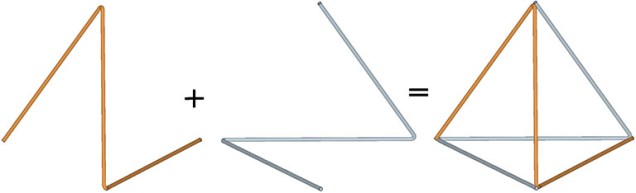
Fuller’s “structural quanta” are related to the idea that all the structural polyhedra can be thought of as self-interfering wave patterns. Each cycle of the wave consists of the three vectors of an open ended triangle. The tetrahedron, for example, consists of two open-ended triangles, one clockwise and one counter-clockwise, as in the following illustration:
The tetrahedron as a self-interfering wave pattern. The waves are represented here as two open-ended triangles (left), one clockwise and one counter-clockwise, which combine to form the four triangles of the tetrahedron (right).
I’ve used the equations described in this topic to calculate the strut and tendon lengths of the tensegrity sphere models I describe in Model Making. They are slightly modified from those published by Hugh Kenner in his book, Geodesic Math and How To Use It (1976, 2003). See also: Tensegrity.
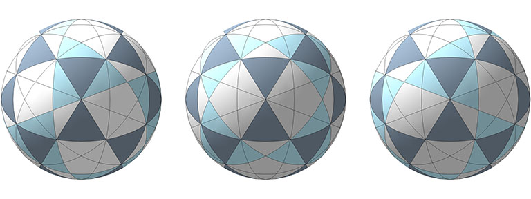
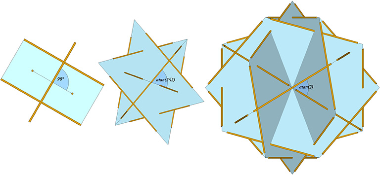
After some rather clever reasoning, Kenner concluded that all of the dimensions of the tensegrity spheres could be derived from just two quantities: the number of sides (n) in their great circle (or lesser circle) planes, and the angle (µ) at which they cross. The following illustration shows the three primary tensegrity spheres, i.e., the spherical phases of the tensegrity tetrahedron, octahedron, and icosahedron:
the six-strut tensegrity sphere with three great circles planes of two struts (n=2), each crossing at µ=90°;
the twelve-strut tensegrity sphere with four great-circle planes of three struts (n=3), each crossing at µ=atan(2√2) ≈ 70.530°; and,
the thirty-strut tensegrity sphere with six great circle planes of five struts (n=5), each crossing at µ=atan(2) ≈ 60.435°.
The great circle planes of the six-, twelve-, and thirty-strut tensegrity spheres, and the angles at which they intersect
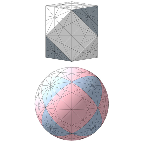
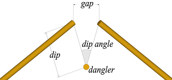
The intersection of the great-circle and lesser-circle planes can be broken down to two struts and a dangler, as in the following illustration.
The gap, dip, and dip angle are parameters used in the calculations for tensegrity structures.
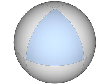
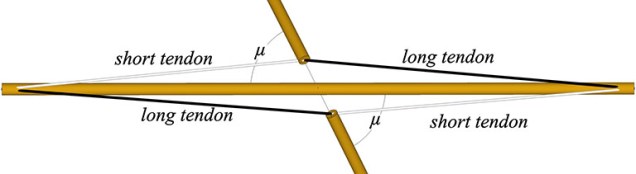
The dangler strut’s great circle crosses the great circle of the other two struts at an angle, µ. If this angle is less than 90° (as is the case for all but the six-strut tensegrity sphere), the tension elements will consist of a long and a short tendon, as shown in the following illustration.
Two struts of a great circle plane crossing the midpoint of a dangler at angle, µ, with the long and short tendons connecting their endpoints.
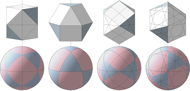
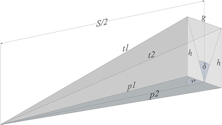
The next illustration shows the relationships between all the parameters that go into calculating the circumsphere radius, strut length, and tendon lengths of the tensegrity spheres:
S = strut length;
r = the circumsphere radius, from sphere center to each of the strut endpoints;
dangler = the strut bisected by the great circle plane of two struts;
μ = the angle the great circle plane of the dangler makes with the great circle plane of the two struts;
d = dip, i.e., the distance between each strut’s endpoint and the midpoint of its dangler;
δ = the dip angle, i.e., the angle between the dangler’s midpoint and the two strut endpoints;
g = the gap, i.e. the linear distance between the two strut endpoints;
h = the vertical distance between a strut’s endpoint and the horizontal plane of its dangler;
t1 and t2 = the length of the short and long tendons, respectively;
p1 and p2 = the base of the right angle made with h, and with t1 or t2 as its hypotenuse, respectively.
Parameters for the equations used to calculate the tendon lengths (t1 and t2) of the three primary tensegrity spheres.