“Complementarity requires that where there is conceptuality, there must be nonconceptuality. The explicable requires the inexplicable. Experience requires the nonexperienceable. The obvious requires the mystical. This is a powerful group of paired concepts generated by the complementarity of conceptuality. Ergo, we can have annihilation and yet have no energy lost; it is only locally lost.“ — R. Buckminster Fuller, Synergetics, 501.13
“…the sum of the angles around each of every local system’s interrelated vertexes is always two cyclic unities less than universal nondefined finite totality. We call this discovery the principle of finite Universe conservation. Therefore, mathematically speaking, all defined conceptioning always equals finite Universe minus two. The indefinable quality of finite Universe inscrutability is exactly accountable as two.” — ibid., 224.50
“Since unity is plural and, at minimum, two, the additive twoness of systemic independence of the individual system’s spinnability’s two axial poles … must be added to something, which thinkable somethingness is the inherent systemic multiplicative twoness of all systems’ congruent concave-convex inside-outness: this additive-two-plus-multiplicative two fourness inherently produces the interrelationship 2 + 2 + 2 sixness (threefold twoness) of all minimum structural-system comprehendibility.” —ibid., 1073.11
At the core of both Fuller’s geometry and his philosophy is the idea that “unity is plural and at minimum two.” You can’t draw a circle without drawing two circles, for example. The circle must be drawn on the surface of some system, and it always divides the system into that which is contained by the circle’s concavity, and that which is contained by the circle’s convexity. The moral point of this concept is that nature has no preference for one over the other. In the math, this essential duality appears as a plus two (the additive two) and the times two (the multiplicative two).
Additive Twoness
For any polyhedron, the sum of its vertices and faces is always equal to its number of edges minus two:
Vertices + Faces = Edges – 2
This is Euler’s topological abundance formula. It can also be written as:
Vertices – Edges + Faces = 2
This same “2” occurs in Fuller’s shell growth formulas for the close-packing of spheres: for any symmetrically close packed array of spheres, the number of spheres in the outer shell is always:
nF²+2
where n is a constant endemic to the system, and F is its frequency, or number of subdivisions along any edge. Fuller attributes this excess of +2 to the poles or spin axis of the system, and sometimes called it the system’s “polarity constant.”
Other examples of the additive two:
A vector has 2 vertices, its starting point and its endpoint.
If the radius of a sphere is taken to be 1, a line drawn between two sphere centers (a single frequency primitive vector connecting two event foci) has a length of 2.
A triangle, or any polygon, has 2 faces, the obverse and the reverse.
Multiplicative Twoness
The formula for the number of spheres in the outer shell of radially close packed spheres is 10F²+2. At zero frequency (F=0) there is only the central sphere, the nucleus. But the formula returns a shell volume of 2 spheres.
10(0)²+2 = 2
The primitive idealized sphere in isolation from other spheres has no defined poles, but it does have two surfaces, its convex outer surface, and its concave inner surface. So, in the case of the single sphere (or any whole system) the +2 has a different meaning, the division of universe into inside and outside, and of polyhedral systems into the concavity enclosing a defined space, and the convexity enclosing the in-definite remainder of the finite universe. This is what Fuller called the “multiplicative two.”
In any omni-triangulated structural system, that is, for any polyhedron structurally stabilized through triangulation: a) the number of vertices (“crossings” or “points”) is always evenly divisible by two (2×1); b) the number of faces (“areas” or “openings”) is always evenly divisible by four (2×2), and; c) the number of edges (“lines,” “vectors,” or “trajectories”) is always evenly divisible by six (2×3). For example, the icosahedron has twelve vertices, twenty faces, and thirty edges. The number of faces is evenly divisible by two (12/2=6); the number of faces is evenly divisible by four (20/4=5); the number of edges is evenly divisible by six (30/6=5). This holds for any polyhedron of whatever size or complexity, just so long as its faces (areas, openings) are triangulated and therefore constitute a “structure” by Fuller’s definition, i.e. any system that holds its shape without external support.
A principle of angular topology (attributed to Descartes) states that the sums of all the angles around all the vertexes of any polyhedron (whether or not it is omni-triangulated and a “structure” by Fuller’s definition) is always 720° less than the number of vertices times 360°. For example, the sum of the angles around the four vertices of the tetrahedron is 720° (4×3×60), 720° less than 1440°, the number of vertices times 360°. Fuller interpreted this to mean that the difference between the non-conceptual and conceptual, the indefinite and the definite, or between infinity and any conceptual system is always one tetrahedron, 360°×2, or two cycles of unity, the multiplicative 2. In fact, the tetrahedron as the miniumum system is emblematic of all the foregoing. Its two (non-polar) vertices, four faces, and six edges are the divisors in the formula for omni-triangulated systems described in the previous paragraph.
“None of the always co-occurring cube’s edges is congruent with the vectorial lines (edges) of the isotropic vector matrix. Thus we witness that while the cubes always and only co-occur in the eternal cosmic vector field and are symmetrically oriented within the field, none of the cubes’ edge lines is ever congruent or rationally equatable with the most economical energetic vector formulating, which is always rational of low number or simplicity as manifest in chemistry. Wherefore humanity’s adoption of the cube’s edges as its dimensional coordinate frame of scientific-event reference gave it need to employ a family of irrational constants with which to translate its findings into its unrecognized isotropic-vector-matrix relationships, where all nature’s events are most economically and rationally intercoordinated with omnisixty-degree, one-, two-, three-, four-, and five- dimensional omnirational frequency modulatability.” —R. Buckminster Fuller, Synergetics, 982.12
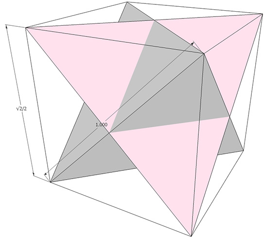
The cube in Fuller’s geometry is conceived as two tetrahedra, one positive and one negative, sharing a common center of volume. In the absence of the triangulation provided by at least one of the tetrahedra, the cube would lack structure and collapse. The length of the face diagonal, rather than the edge length, is therefore taken as unity and produces a cube whose volume is precisely three (3) regular tetrahedra.
The cube, with the face diagonal taken as unit length, d:
6 square faces, 8 vertices, 12 edges
Face angles: all 90°
Dihedral angle: 90°
Tetrahedral volume: 3d³
Cubic volume: d³×√2/4
Surface area (in equilateral triangles): 8d²√3
Surface area (in squares): d²×√2/4
A quanta modules: 48
B quanta modules: 24
In-sphere radius: d×√2/4
Mid-sphere radius: d/2
Circumsphere radius: d×√6/4
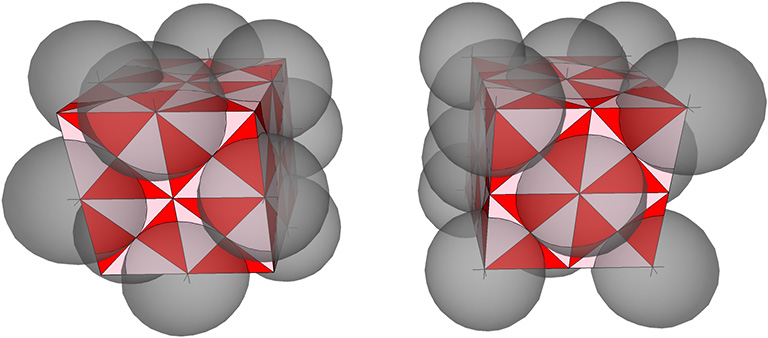
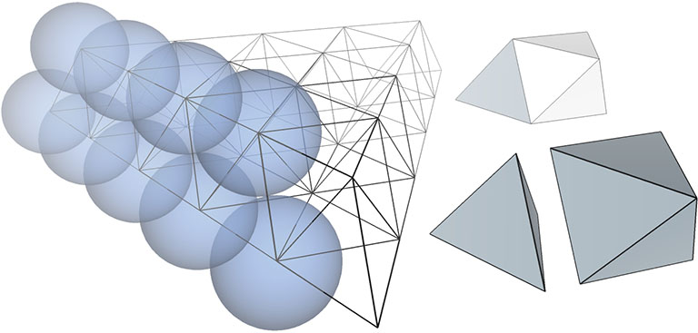
The cube can be constructed from of a regular tetrahedron with four 1/8th octahedra added to its faces.
The volume-3 cube, shown here in quanta modules, is constructed of one regular tetrahedron with four eighth-octahedra added to its faces.
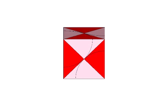
When we model the isotropic vector matrix as vectors between spheres, the volume-3 cube is indistinguishable from the tetrahedron it encloses.
In the vector-sphere model of the isotropic vector matrix, the volume-3 cube is essentially a tetrahedron.
The cube emerges in the isotropic matrix only at higher frequencies, either by adding four tetrahedra centered on the faces of a larger tetrahedron with twice the edge length, or by adding eight tetrahedra to the eight faces of an octahedron with the same edge length.
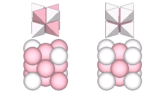
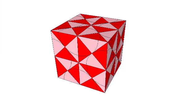
We can stack eight volume-3 cubes in two configurations to form two larger, distinct, cubes, each of volume-24. From the outside, the difference between these two cubes is subtle. What makes each cube unique is the position each occupies in the isotropic vector matrix. The addition of spheres reveals one to be a cube while the other to be a vector equilibrium (VE).
Eight volume-3 cubes can be stacked in two configurations resulting two larger cubes occupying different positions in the isotropic vector matrix.
Dissecting the quanta model reveals the VE to contain eight tetrahedra all sharing a common vertex at the center of the vector equilibrium.
One of the two quanta-module configurations of the the cube reveals eight tetrahedra sharing a common vertex at the center of the VE.
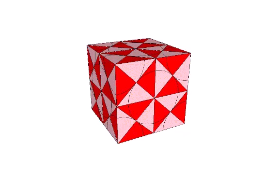
Disecting the quanta model reveals the volume-24 cube to contain eight tetrahedra all rotated at 90° and pointing away from their common center. That is, the two volume-24 cubes constitute the two vector-equilibrium phases of the jitterbug: the VE and the octahedron phases.
The other of the two quanta module configurations of the cube reveals eight tetrahedra rotated 90° away from their common center of volume.
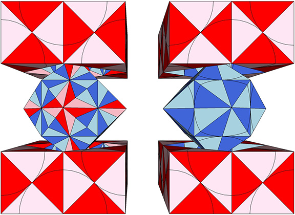
In the quanta model of the isotropic vector matrix, the two cubes overlap. One or the other is revealed depending on how we slice the matrix. When modeled as the radial close packing of spheres, however, the two cubes form discrete modules that close pack to fill the matrix.
The two exchange places during the jitterbug transformation, i.e., one transforms into the other. Each gains or loses a sphere in the process, suggesting the migration of nuclei.
The transformation of the two cubes in the jitterbug suggests the migration of nuclei.
Spheres close pack as cubes in even-numbered layers around octahedra (spaces) and VEs (spheres). In odd-numbered layers, the spheres form partially-truncated cubes surrounding a positive or negative tetrahedron (interstice). The growth pattern repeats every fourth layer, with the first layer surrounding a positive (or negative) tetrahedron; the second layer surrounding an octahedron (or VE); the third layer surrounding a negative (or positive) tetrahedron, and; the fourth layer surrounding a VE (or octahedron).
Close-packed spheres form cubes in even layers with either a sphere or a space at their centers. Odd layers produce partially truncated cubes with either a positive or negative tetrahedron at their centers. The pattern repeats every four layers.
Note that the cube’s edges, no matter the frequency, never align to the vectors connecting sphere centers in the isotropic vector matrix. Only its face diagonals are congruent with the matrix vectors.
Fuller thought that the vector-edged cube and the icosahedron had a combined “energetic” volume (or volume in regular tetrahedra) of 3³, or 27. Actually, their combined volume is just under 27, about 26.997577.
The constant, V, is Fuller’s dymaxion vector constant which equals 2 × ⁶√(9/8), or about 2.039648903. For more information on calculating “energetic” volumes, see Pi and the Synergetics Constants.
The regular icosahedron has an irrational volume in both cubes and tetrahedra. Fuller accounted for this irrationality by noting that the icosahedron exists only as discrete shells and lattices; it does not close pack, either with itself or any other regular polyhedron to fill all space. Nature, therefore, had no need to assign it a volume commensurate with any of the other regular polyhedra.
Its isolation is further reinforced by its axes of spin and the 31 great circles they describe. No great circle unique to the icosahedron passes through any point of contact with spheres radially close-packed in the isotropic vector matrix. Six of its great circles pass through no points of contact, including those between spheres arranged into icosahedral shells and lattices. This isolation suggests the icosahedron to be a model for potential energy, charge, and other holding patterns of energy.
The icosahedron of edge length a has the following properties:
φ=golden ratio, (1+√5)/2)
Face angles: all 60°
Dihedral angle: acos(-√5/3) or 180°-asin(2/3) ≈ 138.189685°;
Central angle of edge: atan(2) ≈ 63.434949°
Volume (in tetrahedra): a³×5φ²√2 ≈ 18.512296
Cubic volume: a³×5φ²/6 ≈ 2.18169499
A and B quanta modules: n/a
Surface area (in equilateral triangles): 20a²
Surface area (in squares): 5a²√3
In-sphere radius: a×φ²√3/6 ≈ 0.755761
Mid-sphere radius: a×φ/2 ≈ 0.809017
Circum-sphere radius: a×(√(φ+2))/2 ≈ 0.9510565
Dihedral and central angles of the regular icosahedron
If the nucleus is removed from a radially close-packed cluster of 13 unit radius spheres (see Vector Equilibrium and the “VE”), the remaining 12 spheres naturally rearrange themselves into the stable configuration of the icosahedron.
Twelve spheres close packed around a central nuclear sphere naturally rearrange themselves into an icosahedron when the central sphere is absent.
The icosahedron is famously derived from the golden ratio (φ), i.e., by connecting the vertices of three golden rectangles arranged orthogonally around a common center.
The regular icosahedron constructed by connecting the vertices of three golden rectangles intersecting at 90° around a common center.
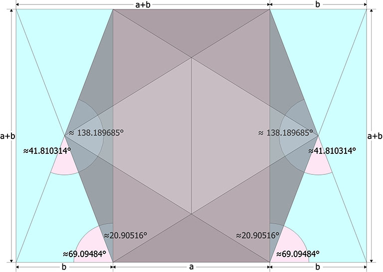
The following illustration shows how the dihedral angles of the regular icosahedron relate to the golden ratio.
The icosahedron’s dihedral angle, about 138.189685°, is equal to 2×arctan(1+φ); its supplementary angle (approximately 41.810315°) is therefore equal to 2×arctan(1/(1+φ)), and that angle’s complementary angle (approximately 69.094846°) is therefore equal to arctan(1+φ).
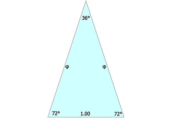
The icosahedron’s circumsphere and mid-sphere radii are the cosines of 18°, (√φ+2)/2, and 36°, φ/2, or the sines of 72° and 54°. The angles 72° and 36° define the golden triangle.
The golden triangle
The two angles of the golden triangle are formed in the icosahedron by a lines drawn perpendicular to the circumsphere or mid-sphere radii and intersecting with a sphere of unit radius, disclosing the relationship between the icosahedron, the unit-radius sphere, and the vector equilibrium (VE).
Perpendiculars drawn from the circumsphere radius (left) and mid-sphere radius (right) of the regular icosahedron intersect with the unit sphere (radius = 1) at angles of 18° and 36° with the radius.
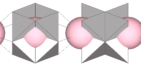
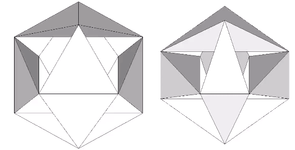
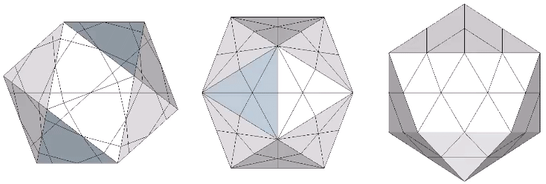
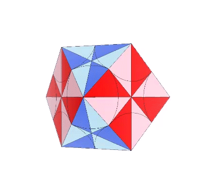
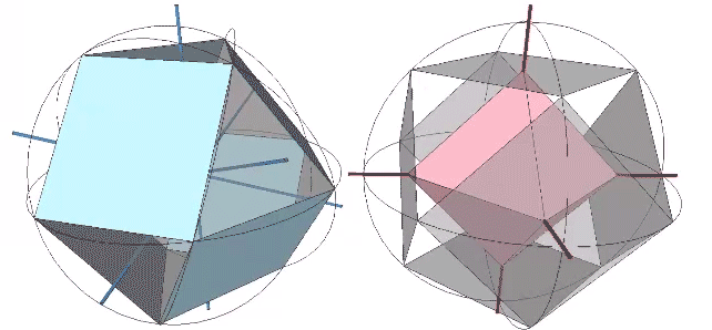
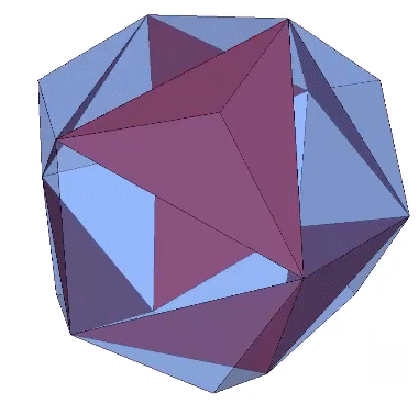
The 36° and 72° angles also show up in the face angles of the polyhedron that complements the icosahedron in the jitterbug transformation, i.e., when the VEs have contracted into the shape of the regular icosahedron, the octahedra have expanded into the shape of its complement, and vice versa. (See: Icosahedron Phases of the Jitterbug.)
The regular icosahedron (gray) and its complement (pink) emerge together in the jitterbug, with the expanding or contracting VEs forming one, and the expanding or contacting octahedra forming the other.
The concave forms of the regular icosahedron and its space-filling complement have, despite their different shapes, identical face angles: eight equilateral triangles (60°, 60°, 60°) and twelve isosceles triangles of 36°, 36°, 54°.
The concave forms of the regular icosahedron and its space filling complement have identical face angles.
We can close up the cavities to create six irregular tetrahedra arranged orthogonally around their common centers. Curiously, the tetrahedral cavities of both the regular icosahedron and its complement have identical, rational cubic volumes of a³/12, or a combined cubic volume of a³/2, where a is the edge length.
Six irregular tetrahedra occupy the cavities of the concave regular icosahedron (left), and its concave complement (right). The combined cubic volume for both is exactly a³/2, where a is the edge length.
The in-sphere radius makes an angle with the mid-sphere radius of atan(2-φ), or about 20.905157°. Some tedious trigonometry works out its length to be φ²√3/6 or about 0.75576131.
In-sphere radius of the icosahedron
The central angle, i.e. the angle between two adjacent vertices of the icosahedron and its center of volume, is the same as the angle from a square’s mid-edge to one of its opposite corners, atan(2), about 63.43894882°.
The angle between two adjacent vertices of the icosahedron and its center of volume is the diagonal of a double square.
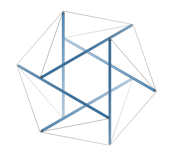
The six-strut tensegrity sphere, sometimes called the “tensegrity icosahedron” or “Jessen Othogonal Icosahedron”, is really a tetrahedron in its tensor equilibrium phase.
The regular icosahedron in its tensor equilibrium phase (left in the figure below) approximates the shape of the icosidodecahedron.
The icosahedron in its tensor equilibrium phase approximates the shape of the icosidodecahedron (left).
All structure is fundamentally reducible to tensegrity, and this applies to the regular icosahedron, shown here transforming between its tensor-equilibrium and polyhedral phases.
The icosahedron has an irrational volume and so is incommensurate with the A and B quanta modules.
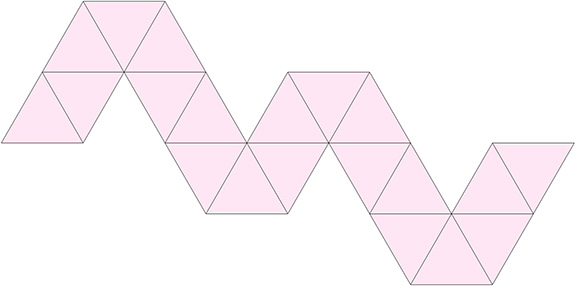
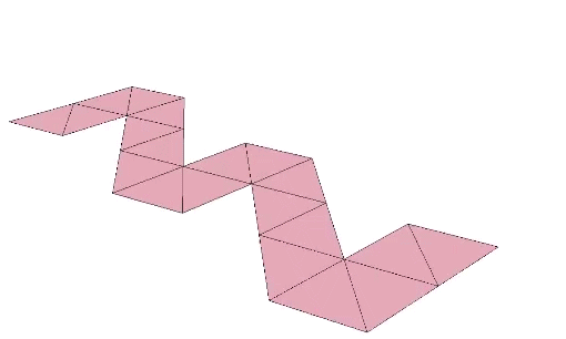
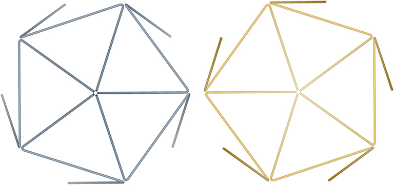
The regular icosahedron can be constructed from a single paper strip of twenty equilateral triangles.
The construction is accomplished by 19 sequential folds of atan(2√5/5).
The regular icosahedron may be constructed from a single paper strip.
The Raleigh Edition of the Dymaxion Airocean World Map (copyright 1954) is a variation of the cartographic projection method Fuller patented in 1946. Earth’s surface is mapped onto the planar facets of the regular icosahedron by a method Fuller called “triangular geodesics transformational projection.” It is one of the most distortion-free maps of the earth’s surface ever devised. Great circles approximate straight lines, and its modules can be rearranged to reveal relationships and orientations not otherwise apparent on more conventional maps.
Fuller’s Dymaxion Airocean World Map, copyright 1954.
The map folds neatly into a regular icosahedron.
Fuller’s Dymaxion Airocean World Map folded into a regular icosahedron.
All the structural (i.e. triangulated) polyhedra may be constructed from an even number triangular helices, or what Fuller called one half of a structural quantum. The tetrahedron and icosahedron (but not the octahedron) require an equal number of clockwise and counter-clockwise helices.
The two helices each occupy their own hemisphere, with exclusively clockwise helices in one hemisphere, and exclusively counter-clockwise helices in the other. Each radiate from diametrically opposed vertices, in effect polarizing the icosahedron on one preferred axis of spin. See also: Isotropic Vector Matrix as Transverse Waves.)
“The 31 great circles of the icosahedron always shunt the energies into local-holding great-circle orbits, while the vector equilibrium opens the switching to omni-universe energy travel. The icosahedron is red light, holding, no-go; whereas vector equilibrium is green light, go. The six great circles of the icosahedron act as holding patterns for energies. The 25 great circles of the vector equilibrium all go through the 12 tangential contact points bridging between the 12 atomic spheres always closest packed around any one spherical atom domain.” — R. Buckminster Fuller, Synergetics, 1132.02
“The six great circles of the icosahedron are the only ones not to go through the potential inter-tangency points of the closest-packed unit radius spheres, ergo energy shunted onto the six icosahedron great circles becomes locked into local holding patterns, which is not dissimilar to the electron charge behaviors.” — ibid. 457.22
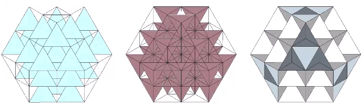
In Fuller’s energetic geometry, the great circles of the VE and icosahedron model energy transference and containment. He described them as “railroad tracks” which either move energy from one domain to another, or divert energy into into loops or holding patterns. Communication occurs when a great circle of one sphere crosses a great circle of an adjacent sphere, i.e. crosses a point of contact or, in Fuller’s terminology, a “kissing point.” All of the 25 great circles of the VE intersect at least two points of contact with neighboring spheres. This is consistent with the role of the VE in the isotropic vector matrix and what Fuller called “nature’s coordinate system.” Of the 31 great circles of the icosahedron, only 7 intersect with the isotropic vector matrix, and these are identical with the sets of 3 and 4 great circles of the VE and the seven axes of symmetry. This isolation is consistent with Fuller’s conception of the icosahedron as a model of potential energy or charge. Of the remaining 24 great circles of the icosahedron, 18 interse ct with adjacent spheres only when close-packed as icosahedral shells, and 6 are true holding patterns, communicating with neither the isotropic vector matrix of radially close-packed spheres, nor with the icosahedron shells of laterally close-packed spheres. (See: Close-Packing of Spheres)
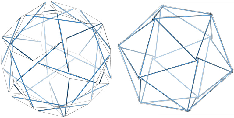
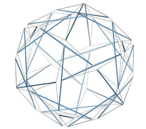
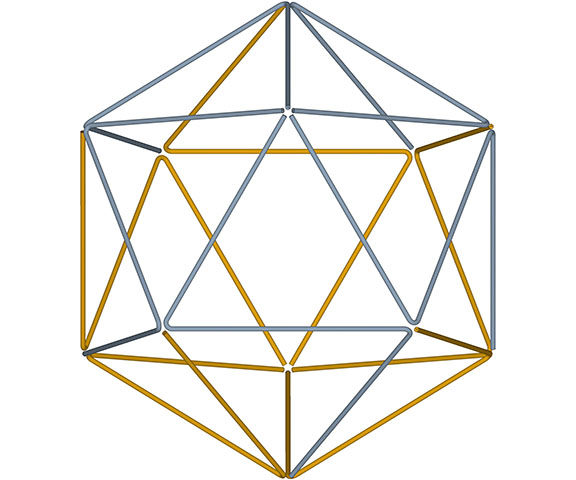
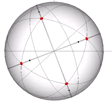
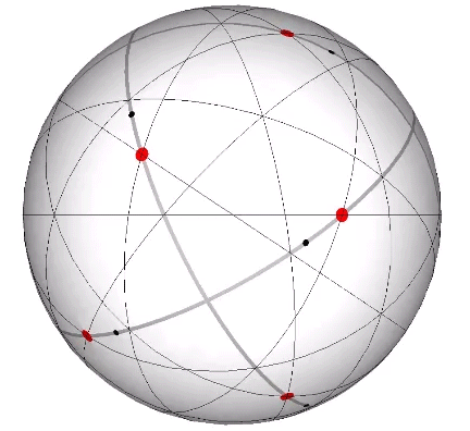
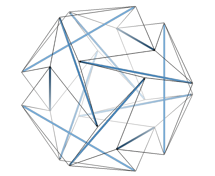
The 31 axes of spin of the icosahedron and their 31 great circles.
The 10 face-to-face axes, the 15 edge-to-edge axes, and the 6 vertex-to-vertex axes define the 31 great circles of the icosahedron.
The 31 great circles of the icosahedron are derived from its 31 axes of spin. Left to right: 10 face-to-face axes; 15 edge-to-edge axes; and 6 vertex-to-vertex axes.
The 31 great circles of the icosahedron disclose the following spherical polyhedra: octahedron; icosahedron; pentagonal dodecahedon; icosidodecahedron; tricontahedron; and VE. See Icosahedron: Spherical Polyhedra Disclosed by Great Circles.
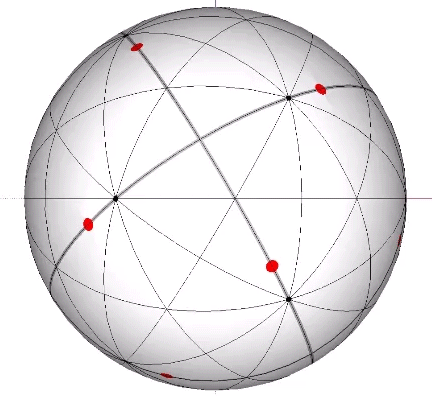
Only seven of the 31 great circles of the icosahedron pass through points of contact between the radially close-packed spheres of the isotropic vector matrix. Their axes are the identical with Fuller’s Seven Axes of Symmetry. These include 4 of the 10 great circles defined by the ten face-to-face axes of the icosahedron (these are the same 4 associated with the VE’s triangular face-to-face axes), and 3 of the 15 great circles defined by the fifteen edge-to-edge axes of the icosahedron (these are the same 3 associated with the VE’s square face-to-face axes). (See: The 25 Great Circles of the Vector Equilibrium.) All of the great circles which are unique to the icosahedron pass through none of the points of contact between the radially close-packed spheres, and are therefore what Fuller called “local-holding great-circle orbits.”
The 15 great circles of the icosahedron each pass through four of the twelve vertices of the icosahedron, and therefore provide communication between spheres close-packed as discrete icosahedron shells or lattices (See: Close Packing of Spheres, and Close Packing of Icosahedra. The 6 great circles of the icosahedron pass through neither the vertices of VE nor those of the icosahedron, and are therefore true holding patterns, providing no inter-sphere communication.
In the figures below, the referenced great circles are indicated by the thin black lines, the points of contact between radially close-packed spheres of the isotropic matrix, or the vertices of the VE, are indicated by red dots. The points of contact between spheres close-packed into discrete icosahedral shells or lattices, or vertices of the icosahedron, are indicted by black dots. The paths followed by the vertices in the jitterbug transformation are indicated by thick gray lines.
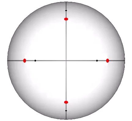
Set of 15 (Axes Connect Opposing Edges)
The 15 great circles defined by the set of fifteen edge-to-edge axes of the icosahedron disclose the spherical pentagonal dodecahedron and the Basic Disequilibrium LCD Triangle. Each of the fifteen great circles passes through four of the twelve vertices of the icosahedron, and each vertex of the icosahedron connects with five great circles. Three of the fifteen pass through the vertices of the VE, and these are identical with the VE’s 3 great circles defined by its three square face-to-face axes of spin.
Three of the icosahedron’s set of fifteen great circles pass through vertices of the VE (red dots) and describe a spherical octahedron. All of the fifteen all pass through the vertices of the icosahedron (black dots)
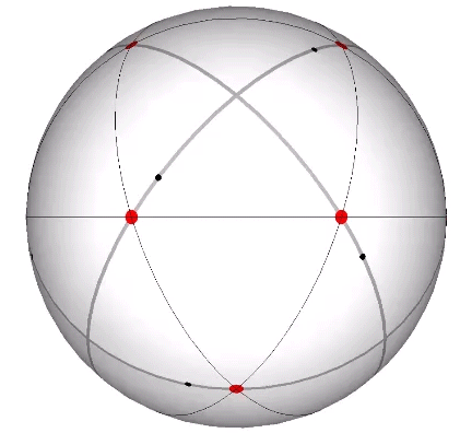
Set of 10 (Axes Connect Opposing Faces)
The 10 great circles defined by the set of ten face-to-face axes of the icosahedron disclose the spherical vector equilibrium (VE). None pass through the vertices of the icosahedron. Four pass through the vertices of the VE, and these are identical with the VE’s 4 great circles which describe the spherical VE.
Four of the icosahedron’s set of ten great circles pass through the vertices of the VE (red dots) and describe the spherical VE. None pass through the vertices of the icosahedron (black dots).
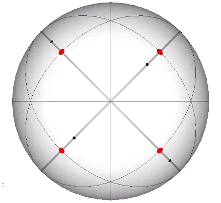
Set of 6 (Axes Connect Opposing Vertices)
The 6 great circles defined by the set of six vertex-to-vertex axes of the icosahedron disclose the spherical icosidodecaheron, the 42-sided polyhedron associated with the spherical form of the 30-strut tensegrity icosahedron. (See: Tensegrity.) None pass through a vertex, neither of the VE nor of the icosahedron, and therefore provide no inter-sphere communication.
None of the icosahedron’s set of six great circles pass through any vertex of the VE (red dots) or the icosahedron (black dots), and are therefore what Fuller called energy holding patterns, providing no inter-sphere communication.
For discussion on the surface and central angles described by the 31 great circles of the icosahedron, see Basic Disequilibrium LCD Triangle.
“The vector equilibrium’s 25 great circles, all of which pass through the 12 vertexes, represent the only most economical lines of energy travel from one sphere to another. The 25 great circles constitute all the possible most economical railroad tracks of energy travel from one atom to another of the same chemical elements. Energy can and does travel from sphere to sphere of closest-packed sphere agglomerations only by following the 25 surface great circles of the vector equilibrium, always accomplishing the most economical travel distances through the only 12 points of closest-packed tangency.” — R. Buckminster Fuller, Synergetics, 452.02
In Fuller’s energetic geometry, the great circles of the VE and icosahedron model energy transference and containment. He described them as “railroad tracks” which either move energy from one domain to another, or divert energy into into loops or holding patterns. Communication occurs when a great circle of one sphere crosses a great circle of an adjacent sphere, i.e. crosses a point of contact or, in Fuller’s terminology, a “kissing point.” All of the 25 great circles of the VE intersect at least two points of contact with neighboring spheres. This is consistent with the role of the VE in the isotropic vector matrix and what Fuller called “nature’s coordinate system.” Of the 31 great circles of the icosahedron, only 7 intersect with the isotropic vector matrix, and these are identical with the sets of 3 and 4 great circles of the VE and the seven axes of symmetry. This isolation is consistent with Fuller’s conception of the icosahedron as a model of potential energy or charge. Of the remaining 24 great circles of the icosahedron, 18 intersect with adjacent spheres only when close-packed as icosahedral shells, and 6 are true holding patterns, communicating with neither the isotropic vector matrix of radially close-packed spheres, nor with the icosahedron shells of laterally close-packed spheres. (See: Close-Packing of Spheres)
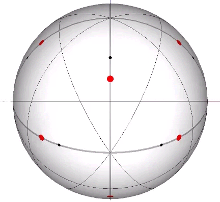
The 25 great circles of the vector equilibrium (VE) are derived from its 25 axes of spin: 12 edge-to-edge axes; 6 vertex-to-vertex axes, 4 triangular-face-to-triangular-face axes; and 3 square-face-to-square-face axes.
The 25 axes of spin of the vector equilibrium and their 25 great circles.
The 25 great circles of the VE are derived from the 25 axes of spin. Left to right: 12 edge-to-edge axes; 3 face-to-face axes (square faces); 4 face-to-face axes (triangular faces); and 6 vertex-to-vertex axes.
All 25 great circles of the VE pass through one or more points of contact between the radially close-packed spheres of the isotropic vector matrix. In the figures below, the referenced great circles are indicated by the thin black lines, the points of contact, or the vertices of the VE, are indicated by red dots. The vertices of the regular icosahedron are indicated by black dots, and the paths the vertices follow in the jitterbug transformation are indicated by gray lines.
Set of 12 (Axes Connect Opposite Edges of VE)
The set of 12 great circles of the VE create a spider web pattern that appears more random than the other great circle sets. In combination with the sets 6 and 4 great circles, the 12 great circles describe an alternate octahedron, but otherwise disclose no other recognizable patterns. Combined, the 12 great circles pass through all 12 points of tangency with neighboring spheres in the isotropic vector matrix.
The set of 12 great circles each pass through 2 of the 12 points of contact with neighboring spheres (red dots).
Set of 6 (Axes Connect Opposite Vertices of VE)
The set of 6 great circles of the VE describe the spherical rhombic dodecahedron, cube, and tetrahedron. Combined, the 6 great circles pass through all 12 points of tangency with neighboring spheres in the isotropic vector matrix.
The set of 6 great circles each pass through 2 of the 12 points of contact with neighboring spheres (red dots).
Set of 4 (Axes Connect Opposing Triangular Faces of VE)
The set of 4 great circles of the VE describe the spherical vector equilibrium. Each intersects with 6 points of tangency with neighboring spheres in the isotropic vector matrix, and the set as a whole passes through all 12 points of tangency. The set of 4 great circles in combination with the set of 3 great circles of the VE comprise the seven axes of symmetry.
The set of 4 great circles each pass through 6 of the 12 points of contact with neighboring spheres (red dots).
Set of 3 (Axes Connect Opposing Square Faces of VE)
The set of 3 great circles of the VE describe the spherical octahedron. Each intersects with 4 points of tangency with the isotropic vector matrix, and the set as a whole intersects with all 12 points of tangency. The set of the 3 great circles in combination with the set of 4 great circles of the VE comprise the seven axes of symmetry.
The set of 3 great circles each pass through 4 of the 12 points of contact with neighboring spheres (red dots).
“When the centers of equiradius spheres in closest packing are joined by most economical lines, i.e., by geodesic vectorial lines, an isotropic vector matrix is disclosed, ‘isotropic’ meaning “everywhere the same,” ‘isotropic vector’ meaning “everywhere the same energy conditions.” This matrix constitutes an array of equilateral triangles that corresponds with the comprehensive coordination of nature’s most economical, most comfortable, structural interrelationships employing 60-degree association and disassociation. Remove the spheres and leave the vectors, and you have the octahedron-tetrahedron complex, the octet truss, the isotropic vector matrix.” — R. Buckminster Fuller, Synergetics, 420.01
“Euclid was not trying to express forces. We, however … are exploring the possible establishment of an operationally strict vectorial geometry field, which is an isotropic (everywhere the same) vector matrix. We abandon the Greek perpendicularity of construction and find ourselves operationally in an omnidirectional, spherically observed, multidimensional, omni-intertransforming Universe.” — ibid. 825.28
The vector equilibrium (VE) and the isotropic vector matrix constitute the core of Fuller’s geometry. Its discovery is one of Fuller’s earliest memories, from a kindergarten class in his childhood home of Milton, Massachusetts. Given semi-dried peas and toothpicks, and a visual deficit as yet uncorrected by the strong glasses he wore all his life, he fumbled sightlessly, and through touch alone constructed what he would later name the octet truss. His classmates constructed cubes and the gabled house-like shapes they were familiar with. Fuller constructed something that satisfied his sense of touch rather than his sense of sight, a sense which could easily have been prejudiced by the cubes and right angles of his built environment. Instead, his fingers naturally sought out and found the triangle, the tetrahedron, and the octahedron, arrangements which, unlike squares and cubes, held their shape and could not be deformed. He credits his kindergarten teacher, Miss Parker of Milton, Massachusetts, with the discovery; it was her praise and kind remarks that fixed the experience in his memory and, eventually, would inspire a lifelong critique of conventional geometry, and his explorations into the energetic-synergetic geometry of nature.
The isotropic vector matrix is formed by connecting the centers of uniform, radially close-packed spheres. Removing the spheres and leaving only the lines (vectors) between them reveals a complex of octahedra and tetrahedra, i.e., the octet truss.
The isotropic vector matrix is the geometric analog to Fuller’s more general statement of Avogadro’s proposition, that “under identical, unconstrained, and freely self-interarranging conditions of energy all elements will disclose the same number of fundamental somethings per given volume.” Fuller’s geometry replaces the abstract concept of infinite lines and line segments with the physical concept of energy vectors. A geometric model of Avogadro’s equilibrium state must have all energy vectors of equal length, i.e. equal products of mass times velocity, and all interacting at the same angles. All vectors in the isotropic vector matrix therefore are of equal length, i.e. the diameter (or two times the radius) of the uniform sphere, and all interact with the others at exactly 60°.
Construction can be accomplished by vertex-bonded (positive or negative) tetrahedra, or by edge-bonded octahedra. Positive-tetrahedron or negative-tetrahedron constructions (but not both) produce a matrix of single vectors, while the octahedron constructions produce a matrix of doubled vectors. Edge-bonding positive and negative tetrahedron together produces a doubled-vector matrix complementary to the doubled-vector octahedron construction.
Each of the two constructions (edge-bonded positive and negative tetrahedra, and edge-bonded octahedra) can be transformed into the other by turning themselves inside out. Note that this inside-out transformation results in the same matrix, one emphasizing the tetrahedra and the other emphasizing the octahedra; there is no shifting of vertices or exchanging of spheres and spaces as in The Jitterbug transformations.
The isotropic vector matrix consists of tetrahedra with octahedron spaces, or of octahedra with tetrahedron spaces. One transforms into the other suggesting that the octahedron may be understood as a positive-negative pair of tetrahedra turned inside out.
All of the models of the isotropic vector matrix can be broken down into the following:
spheres,
spaces, and;
interstices.
In the vector model, the sphere is represented by the vector equilibrium (VE), the space by the octahedron, and the interstices by positive and negative tetrahedra. In the quanta model, spaces and spheres are represented by the two constructions of rhombic dodecahedron, and the interstices appear as tetrahedra or cubes. In the spheres and interstitial models, the spheres are represented, obviously, by spheres, the spaces are represented by concave VEs inside of the octahedra, and the interstices are represented as concave octahedra inside of the tetrahedra.
The isotropic vector matrix consists of spheres (left); interstices (middle); and spaces (right). Each is shown as it is represented in the vector model (top), quanta model (middle), and as radially close-packed spheres (bottom).
The second definition applies to a subset of the first. Fuller noted that truncations through the vertices and edges of the regular tetrahedron produces a tetrakaidecahedron with six square and eight hexagonal faces. (Truncating the faces will produce only a smaller tetrahedron.) The tetrakaidecahedron has fourteen faces, lines through the centers of which define seven axes of spin. Coordinated truncations produce the Kelvin truncated octahedron, which is associated with nuclear domains in the isotropic vector matrix, and with the optimal cellular packing of the Weaire-Phelan matrix (see Tetrakaidecahedron and Pyritohedron).
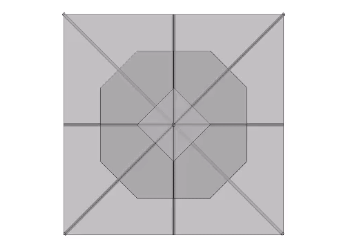
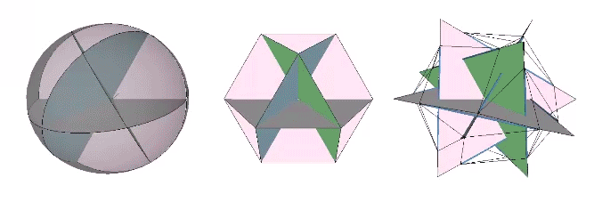
The Seven Axes of Symmetry are identical with the seven face-to-face axes of the VE, and correspond to four of the icosahedron’s ten face-to-face axes and three of its fifteen edge-to-edge axes. The great circles defined by the set of 4 axes discloses the spherical VE (red in the figure below), and the great circles defined by the set of 3 axes defines the spherical octahedron (blue in the figure below).
The great circles defined by the Seven Axes of Symmetry disclose the spherical vector equilibrium (pink) and spherical octahedron (blue).
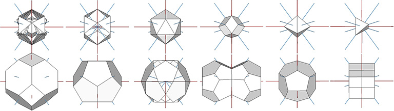
All the regular polyhedra, as well as other polyhedra significant to Fuller’s geometry, align with the Seven Axes of Symmetry.
All regular polyhedra, and more, align with the Seven Axes of Symmetry. Top row, left to right: Jitterbug phases; VE; Icosahedron; Rhombic Dodecahedron; Octahedron; Tetrahedron. Bottom row, left to right: Kelvin Truncated Octahedron; Pentagonal Dodecahedron; Icosidodecahedron; Paired Tetrakaidecahedra in the Weaire-Phelan Matrix; Pyritohedron; Cube.
“The tetrakaidecahedron (Lord Kelvin’s “Solid”) is the most nearly spherical of the regular conventional polyhedra; ergo, it provides the most volume for the least surface and the most unobstructed surface for the rollability of least effort into the shallowest nests of closest-packed, most securely self-cohering, allspace- filling, symmetrical, nuclear system agglomerations with the minimum complexity of inherently concentric shell layers around a nuclear center.“ —R. Buckminster Fuller, Synergetics, 942.70
The Kelvin truncated octahedron, or Kelvin, is a space-filling, fourteen-sided polyhedron with eight hexagonal faces and six square faces, all of equal edge-length. It got its name from a problem posed by Lord Kelvin in the 19th century, to find an arrangement of cells of equal volume so that their total surface area is minimized.
The six vertices of the regular octahedron (left) are truncated to create the six square faces of the Kelvin (right).
Note: Fuller refers to this shape as the tetrakaidecahedron, a generic term for all 14-sided polyhedra. I reserve this term for the all-space filling complement to the pyritohedron in the Weire-Phelan matrix. See Tetrakaidecahedron and Pyritohedron.
This truncated octahedron was proposed by Lord Kelvin as the solution to the Kelvin problem: How can space be partitioned into cells of equal volume with the least area of surface between them?
Angles and dimensions of the Kelvin tetrakaidecahedron or truncated octahedron with edge length a:
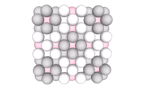
The fourteen sided Kelvin Structure encloses nuclear domains in the radial close-packing of unit-radius spheres.
Presently the best solution to the Kelvin problem is the Weaire-Phalen matrix, consisting of pyritohedra and tetrakaidecahedra. Perhaps not surprisingly, the Kelvin can be derived from from this matrix. Connecting radials of the tetrakaidecahedra forms the very same Kelvin as above. Its edges are of unit-length, the same as the spheres’ diameters.
Connecting the radials of the tetrakaidecahedra in the Weaire-Phelan matrix defines the nuclear domain as the Kelvin truncated octahedron
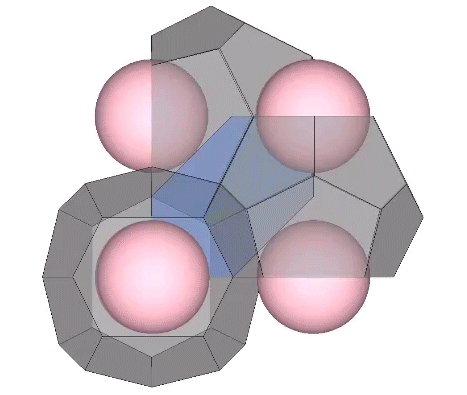
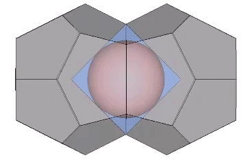
It may be easier to see how the Kelvin faces are derived from the radials of the tetrakaidecahedron if we examine one of its square faces and one of its hexagonal faces individually. The pink spheres in the illustrations below are the non-unique nuclei, those nuclei whose shells are shared with their neighbors. See Formation and Distribution of Nuclei in Radial Close-Packing of Spheres.
Connecting the radials of three adjacent tetrakaidecahedra (face-bonded on their elongated pentagonal faces) describes the hexagonal face of the Kelvin.
Connecting the radials of two adjacent tetrakaidecahedra (face-bonded on their hexagonal faces) describes the square face of the Kelvin.
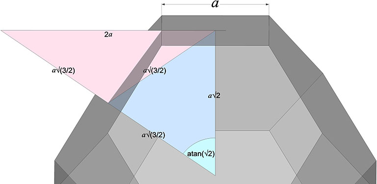
The two in-sphere radii—from center to mid-square-face, and from center mid-hexagonal-face—make an angle of arctan(√2) ≈ 54.735610° with each other. A line drawn between the mid-faces creates an isosceles triangle with a base of a√2 and sides of a√(3/2). Extending the mid-hexagon-face radius to where it crosses a line drawn perpendicular from the mid-square-face radius creates an isosceles triangle with a base of 2a (where a = edge length, unity, or sphere diameter) and sides of a√(3/2). Combining the two isosceles triangles creates a right triangle whose legs measure a√2 and 2a, and whose hypotenuse measures 2×a√(3/2) = a√6.
The two midsphere radii form an isosceles triangle. Extending the mid-hexagon-face to precisely twice its length forms a right triangle with a perpendicular to the mid-square-face radius.
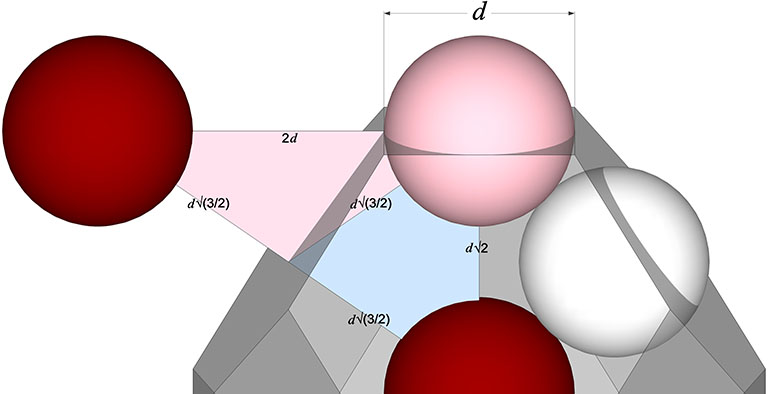
This triangle maps to the distribution of nuclei in the isotropic vector matrix, with unique nuclei centered on the vertices of the two non-right angles, and the nuclei that share their shells with adjacent nuclei centered on the right angle’s vertex.
Note that in the illustrations below, d = a = the sphere diameter. Unique nuclei are colored red, non-unique nuclei are pink, and the spheres occupying the shells of nuclei are white.
The corners of the right triangle formed from the midsphere radii coincide with the centers of nuclei in the isotropic vector matrix.
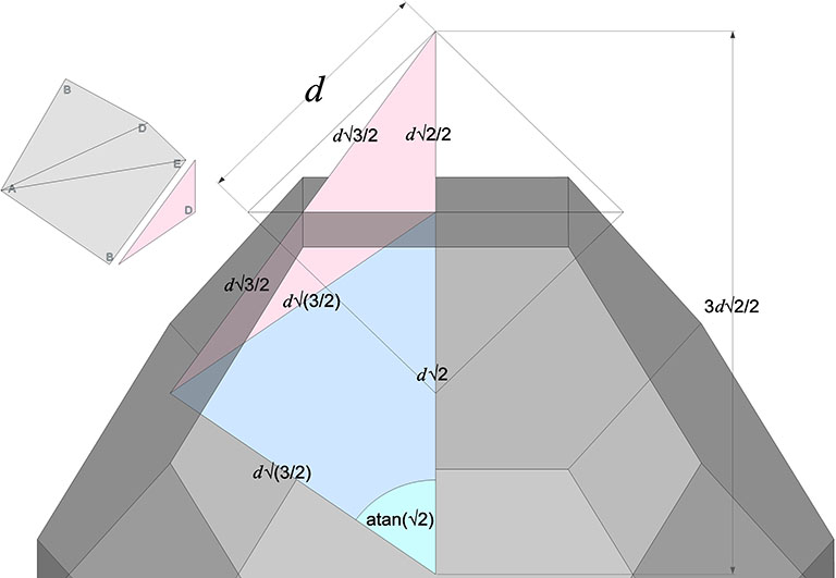
Extending the mid-square-face radius to a point where it crosses a line drawn perpendicular to the mid-hexagon-face radius creates a scalene triangle whose angles are curiously identical with the interior face of the B quanta module. Combining this scalene triangle with the isosceles triangle mentioned above creates a right triangle whose legs measure 2d√2/2 and d√(3/2). The mid-square-face radius extends d√2/2 beyond the face, exactly half of the face’s diagonal length, and half the mid-square-face radius. This suggests a rotational transformation of the Kelvin that may shadow the space-to-sphere, sphere-to-space transformations of the isotropic vector matrix, something begging to be investigated further, along with that curious appearance of the interior face of the B quanta module (pink in the illustration below).
Extending the mid-square-face radius to a point where it crosses the perpendicular to the mid-hexagon-face radius forms a scalene triangle exactly proportional to the interior face of the B quanta module (inset upper left).
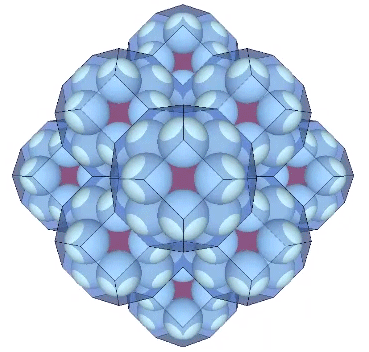
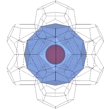
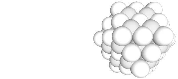
If we replace the twelve vertices of a one-frequency Kelvin with spheres, we find that they occupy the spaces between the 42 spheres of the two 2-frequency vector equilibrium (VE) shell. The 2-frequency VE is significant because its shell is the last to fully enclose the nucleus without containing any new potential nuclei. The 1-frequency Kelvin complements the 2-frequency VE to fully isolate unique nuclear domains.
The one-frequency Kelvin occupies the spaces between the spheres of the two-frequency VE and fully isolates the nucleus.
Kelvins with even frequencies (odd numbers of spheres to the side) are coincident with the radially close-packed spheres of the isotropic vector matrix. Those with odd frequencies (even numbers of spheres to the side) occupy the spaces between radially close-packed spheres.
Kelvins of even frequencies (white spheres) are coincident with the spheres of the isotropic vector matrix. Kelvins of odd frequencies (gray spheres) occupy the spaces between them.
At the center of odd Kelvins is a space, i.e., concave VE, and at the center of even Kelvins is a sphere. Note that the odd Kelvins in the above examples which fully isolate the nucleus have been shifted by 1/2 of a sphere diameter out of their natural position in the matrix. (See also: Spaces and Spheres (Redux), and; Spheres and Spaces.)
Fuller used the Kelvin to illustrate his seven axes of symmetry which he derived from the truncations of the tetrahedron’s four vertices and six edges.
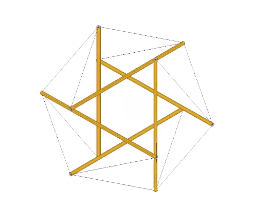
Fuller’s conception of the Kelvin as a truncated tetrahedron, rather than a truncated octahedron, is perhaps due to its association with the spherical form of the tensegrity tetrahedron, the six-strut tensegrity sphere or Jessen Orthogonal Icosahedron.
The six-strut tensegrity sphere (middle) is constructed by joining two-each vertices from opposing square faces of the Kelvin (left). The Jessen orthogonal icosahedron (right) describes its polyhedral shape.
“The geometrical model of energy configurations in synergetics is developed from a symmetrical cluster of spheres, in which each sphere is a model of a field of energy all of whose forces tend to coordinate themselves, shuntingly or pulsatively, and only momentarily in positive or negative asymmetrical patterns relative to, but never congruent with, the eternality of the vector equilibrium. “ — R. Buckminster Fuller, Synergetics, section 205.01
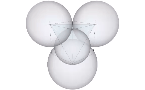
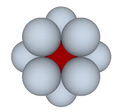
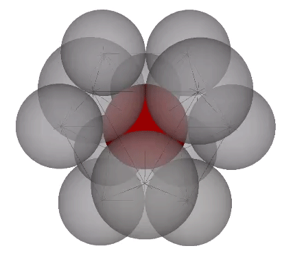
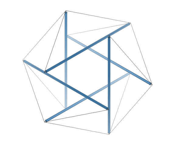
Vectors connecting the centers of unit-radius spheres clustered around a common nucleus define the VE, or vector equilibrium.
The vectors connecting the centers of unit-radius spheres clustered around a common nucleus define the vector equilibrium (“VE”).
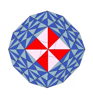
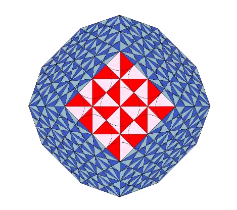
In the VE, the number of modular subdivisions, i.e. frequency, of the radii is exactly the same as the number of modular subdivisions of the chords. Frequency may refer, then, to the number of shells surrounding the nucleus or to the number of subdivisions of any edge vector.
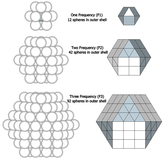
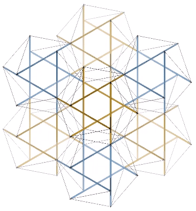
The radial close packing of equal radius spheres about a nuclear sphere forms vector equilibria of progressively higher frequencies. The number of spheres in the outer shell is always the frequency (F)—the number of subdivisions of the radial or edge vectors running through the sphere centers—raised to the second power, which is then multiplied by ten, then added to two, or 10F²+2. In the illustration below, the F1 VE (with unit radial and edge vectors) has twelve spheres in its outer shell: (10×1)+2=12. The F2 VE (whose radial and edge vectors have been divided into two subdivisions) has 42 spheres in its outer shell: (10×2²)+2=42. The F3 VE (with three subdivisions) has 92 spheres in its outer shell: (10×3²)+2=92.
Shell Volume (in spheres or vertices) of VE = 10F²+2
Equal radius spheres close-pack as a matrix of vector equilibria of progressively higher frequencies. The number of vertices or spheres in any layer is given by the formula 10F²+2.
The cumulative number of spheres in a radially close-packed array is therefore:
10(F12+F22+F32+ … +Fn2)+2Fn+1,
which integrates to:
(20F3+30F2+22F+6)/6
The polyhedral shape of these nuclear assemblages of closest-packed spheres is always that of the vector equilibrium, having always six square, and eight triangular faces, for a total of fourteen. The square faces are the equatorial sections of six half-octahedra, and the triangular faces are the bases of eight tetrahedra. If the tetrahedron is taken as unity, the volume of the vector equilibrium is twenty (20). The volume in tetrahedra of any series of vector equilibria of progressively higher frequencies is always frequency to the third power times 20.
Volume (in tetrahedra) of VE = 20F³
The VE is the only construction of radially close-packed spheres that produces uniform and uninterrupted layers. Radial close-packing as octahedra is achieved only with even-numbered layers (odd numbered layers are centered on spaces), and radial close packing as tetrahedra and cubes is achieved only with every other even layer (odd numbered layers are centered on either a positive or a negative tetrahedron, and every other even layer is centered on a space).
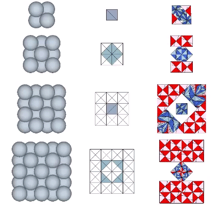
In A and B quanta modules, the VE of frequency, F, equal to 1 consists of 336 A quanta modules and 144 B quanta modules for a total of 480 quanta, a volume of 480÷24=20 tetrahedra.
The quanta module model of the F1 vector equilibrium constructed of eight tetrahedra, with 24 A quanta modules each, and six half octahedra, with 24 A and 24 B quanta module each, for a total volume of 480 quanta modules.
The polyhedron associated with the external shape of the VE is conventionally recognized as the cuboctahedron, or the truncated cube. That its edge lengths are identical to the length of its circumsphere radii was perhaps less well known, and its association with the radial close-packing of unit-radius spheres was either unknown or dismissed by mathematicians as of peripheral interest. For Fuller, these characteristics were central to his search for the geometric analog to his more general statement of Avogadro’s proposition, that under under identical, unconstrained, and freely self-interarranging conditions of energy all elements will disclose the same number of fundamental somethings per given volume. This was discovered to be his octet truss, or isotropic vector matrix, and the vector equilibrium (VE) is its metonymous form.
The question of structure, too, has historically been peripheral to the study of pure geometry; the subject was left to the engineers, and the engineers had for millennia been mostly stone masons for whom one geometric shape was as solid as the next. Fuller’s octet truss and geodesic structures were unknown until the “space age” of the mid-twentieth century. In the absence of its radial vectors, the remaining circumferential (edge) vectors of the cuboctahedron are left unsupported and will collapse, just as the vector model of the cube it was based on will collapse without additional triangulation. Neither is structural, if by “structure” we mean something that holds its shape without external support. In the absence of gravity and the solid earth beneath them, few man-made structures fit this definition.
A third point of contention that Fuller had with conventional geometry was its attention to linear growth and parallel lines, which he attributed to our flawed notion of a flat earth that extended to infinity, and a single direction for “up,” the equal and opposite direction of our “down-to-earth” sensibilities. Nature, if unconstrained, prefers radial (outward-inward) growth with circumferential (precessional-perpendicular) constraints.
The 12-strut tensegrity sphere approximates the overall shape of the VE, and perfectly models what Fuller meant by this. Like all his tensegrities, its structural integrity is maintained by a balance between the radial compression of its struts, and the circumferential tension of its tendons. The twelve-strut tensegrity sphere will torque naturally into the tensegrity octahedron, a transformation recapitulated in the vector model of the jitterbug.
The 12-strut tensegrity sphere approximates the shape of the VE and torques naturally into the tensegrity octahedron.
The VE consists of four great circles, i.e., four 3-strut triangles in the twelve-strut tensegrity sphere, or four hexagons in the vector model.
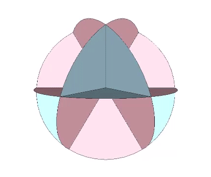
The VE consists of four great circles with axes running through its triangular faces. The 12-strut tensegrity sphere (right) approximates the shape of the VE with each great circle defined by three-strut triangles.
It is likely no coincidence that the surface area of the sphere is equal to the combined surface areas of the VE’s four great-circle disks. The two sides of each disk account for both the convex external surface of the sphere and its concave internal surface. (See: Anatomy of a Sphere.) In the bow-tie construction of the VE, produced by folding the great circle disks along the VE’s central 60° angles, both surfaces are exposed, one inside the square faces, the convex, energy-dispersing surface, and the other inside the triangular faces, the concave, energy-focusing surface. This interpretation of the bow-tie model is strengthened by the quanta model in which the square faces expose the energy-dissipating B modules, and the triangular faces expose the energy-conserving A modules. (See: A and B Quanta Modules.)
Bow-tie construction of the VE, made from the four great circle disks of VE’s 4 triangular-face-to-face axes of spin.
The Seven Axes of Symmetry common to all the regular polyhedra correspond to the 4 axes of spin running through the VE’s eight triangular faces, plus the 3 axes running through its six square faces, the former disclosing spherical VE and its four great circles, and the latter disclosing the spherical octahedron and its three great circles.
The Seven Axes of Symmetry correspond to the VE’s 4 triangular and 3 square face-to-face axes of spin, whose great circles disclose the spherical VE and the spherical octahedron.
Transformations of the VE disclose the regular icosahedron, the Jessen icosahedron (or six-strut tensegrity sphere), the regular octahedron, and the regular tetrahedron. The transformation to the regular icosahedron is perhaps best modeled in the radial close packing of spheres. With the removal of the central sphere, the twelve remaining spheres naturally reposition themselves into the shape of the icosahedron.
With the central sphere removed, the remaining twelve spheres of the VE’s shell rearrange themselves into an icosahedron.
The transformation to the Jessen orthogonal icosahedron is perhaps best modeled in the jitterbugging of the six-strut tensegrity, or tensegrity tetrahedron which, in its most relaxed, spherical, or equilibrium state is identical with the Jessen icosahedron.
The Jessen Orthogonal Icosahedron is identical with the 6-strut tensegrity sphere, and occurs at the precisely midway between the VE and octahedron phases of the jitterbug transformation.
The transformation to the regular octahedron is disclosed through torquing of the 12-strut tensegrity (see above), but is perhaps most convincingly modeled in the jitterbug transformation by the coordinated rotations of its eight triangular faces.
The conventional model of the jitterbug, with the VE transforming into the octahedron and vice versa.
The transformation of the VE into the regular tetrahedron can be accomplished in the vector model by adding a 180° twist to the downward motion of the jitterbug.
Adding a 180° twist to the jitterbug bypasses the octahedron phase and results in the transformation of the VE into the tetrahedron.
But the transformation of the VE into a tetrahedron is perhaps best modeled in the six-strut tensegrity sphere (aka Jessen icosahedron) which occurs at the precise midpoint of the jitterbug transformation. (See: Icosahedron Phases of the Jitterbug.) From here, the VE may continue its transformation into the octahedron, or it can be torqued into the shape of a regular tetrahedron. A clockwise or counter-clockwise torque will produce either a positive or a negative tetrahedron. (See: The Dual Nature of the Tetrahedron.)
The six-strut tensegrity sphere can be torqued either clockwise or count-clockwise to produce the positive or the negative tetrahedron.
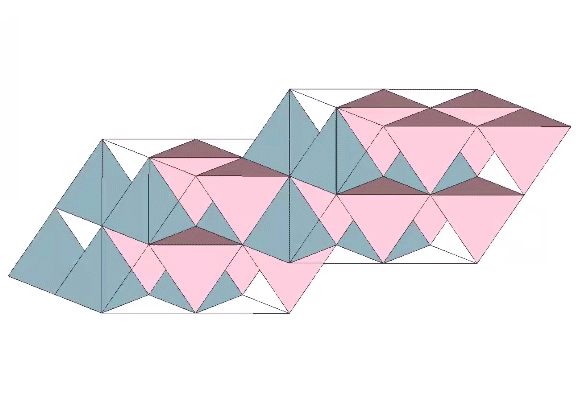
For me, the most compelling model of the jitterbug transformation, which Fuller identified with wave-particle duality, the equivalence of mass and energy, the balance of disintegrative, radiational forces (compression) with integrative, gravitational forces (tension), and which he intuited as a generative metaphor for nearly everything in the physical sciences, if not for everything that is thinkable, is the following: eight, six-strut tensegrity spheres surrounding a common center, and transforming between positive and negative tetrahedra.
This model is illustrated below, with four of the eight, six-strut tensegrity spheres torquing clockwise to form the positive tetrahedron, and the other four torquing counter-clockwise to form the negative tetrahedron, which then switch roles to reverse the process. The result is an oscillation between the VE, with the eight tetrahedra all sharing a common vertex at its center, and the octahedron, with the eight tetrahedra projecting from its eight faces. In the context of the isotropic vector matrix, all the vertices of all the tetrahedra always converge on the center of a VE, but these convergences shift by one-half wavelength with each cycle, exchanging the nuclear spheres (vertex convergences) at the centers of the VEs, with the nuclear space at the centers of the octahedra. (See also: Spheres and Spaces.)
Eight six-strut tensegrity spheres transforming between positive and negative tetrahedra is perhaps the most accurate model of Fuller’s “Jitterbug Transformation.”
“The tetrakaidecahedron develops from a progression of closest-sphere-packing symmetric morphations at the exact maximum limit of one nuclear sphere center’s unique influence, just before another nuclear center develops an equal magnitude inventory of originally unique local behaviors to that of the earliest nuclear agglomeration.“ — R. Buckminster Fuller, Synergetics, section 942.71
The tetrakaidecahedron that Buckminster Fuller had in mind, and which he refers to as “Lord Kelvin’s Solid” was the truncated octahedron, a polyhedron which, like the vector equilibrium (VE), has fourteen sides, and which at the time (1975) was considered the tentative solution to the Kelvin Problem: How can space be partitioned into cells of equal volume with the least area of surface between them? Fuller, like most others, assumed that a bitruncated cubic honeycomb consisting of truncated octahedron cells was, with only slight deformation, the most likely solution. Ten years after Fuller’s death, in 1993, Denis Weaire of Trinity College Dublin and his student Robert Phelan showed through computer simulations of foam that a combination of pyritohedra and tetrakaidecahedra of equal volume could fill space more efficiently, with a surface area to volume ratio 0.3% less that that of Kelvin’s truncated octahedra.
There is a curious correlation between the close packing of unit-radius spheres and foams of unit-volume cells. Spheres close pack around a central sphere as vector equilibria of increasing frequency. The polyhedral domain of each sphere is a rhombic dodecahedron. Rhombic dodecahedra close pack exactly as spheres close pack, twelve around one. (See The Rhombic Dodecahedron.) If we partition close-packed spheres into nuclear domains of central spheres surrounded by unique 12-sphere shells, the shells are distributed as Kelvin’s tetrakaidecahedra, but the nuclei themselves are distributed exactly as the pyritohedra are distributed in the Weaire-Phelan matrix. See: Formation of New Nuclei in Close-Packing of Spheres.
Both the bitruncated cubic honeycomb consisting of truncated octahedra, and the Weaire-Phelan matrix consisting of pyritohedra and tetrakaidecahedra, isolate unique nuclei in the close-packed spheres of the isotropic vector matrix. In the figure below, the isolated nuclei are shown as red spheres, and those that share their shells with neighboring nuclei are shown as pink spheres. In the top row, the vector equilibria of the isotropic vector matrix surround both the red and pink nuclei; they do not distinguish unique nuclei. The truncated octahedra in the middle row do distinguish unique nuclei if their edge length is equal to the sphere diameter, with every other nuclear domain sharing a common center with a truncated octahedron. The Weaire-Phelan matrix (bottom row) distinguishes unique nuclei by their own polyhedron, the pyritohedron, while those that share their shells with neighboring nuclei are centered between positive and negative tetrakaidecahedra. The tetrakaidecahedra are sized so that their circumsphere radius is equal the the sphere diameter.
In the isotropic vector matrix (top row), all nuclear spheres are enclosed within VE’s, whether or not their shells are shared with neighboring spheres. Kelvin truncated octahedra (middle row) distinguish between unique nuclei (red) and those sharing their shells with neighboring nuclei (pink). The Weaire-Phelan matrix (bottom row) distinguishes unique nuclei as those sharing a common center with the pyritohedra.
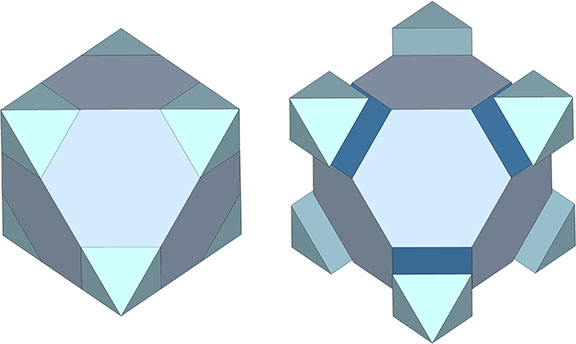
The pyritohedron is familiar as its namesake, the pyrite crystal, or “fool’s gold,” which like the regular dodecahedron has twelve identical faces. The pentagonal faces of the pyritohedron are irregular, with one edge slightly longer that the other four. The pyritohedron can be derived from the Jessen Orthogonal Icosahedron, more familiar in Fuller’s geometry as the convex shape of the six-strut tensegrity sphere. The correlation is intriguing. See also: Tensegrity, and Icosahedron Phases of the Jitterbug.
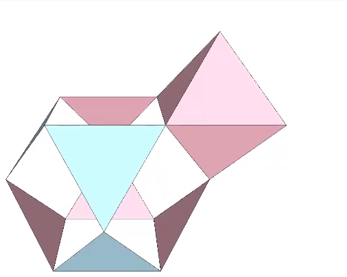
The pyritohedron (clear blue) can be derived from the Jessen Orthogonal Icosahedron (red), the polyhedral shape of the six-strut tensegrity sphere.
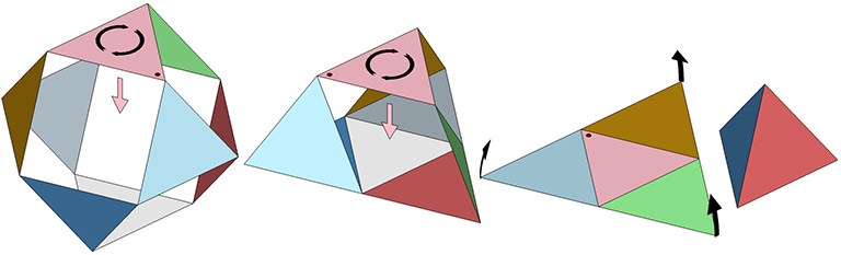
The pyritohedron can be constructed by the addition of eight shallow tetrahedra to each of the eight equilateral triangles of the Jessen icosahedron. The height of these tetrahedra is exactly 1/3 the in-sphere radius of the Jessen icosahedron, or one quarter the circumsphere radius of the pyritohedron.
Adding eight shallow tetrahedra to the equilateral triangles of the Jessen Icosahedron (the polyhedral domain of the six-strut tensegrity sphere) forms the pyritohedron. The height of the tetrahedra is 1/3 the in-sphere radius of the Jessen Icosahedron, or 1/4 the circumsphere radius of the pyritohedron.
An even more beautiful symmetry, I think, is disclosed by connecting the peaks of the eight shallow tetrahedra to form a cube.
Connecting the peaks of the eight shallow tetrahedra forms a cube disclosing rational symmetry with both the pyritohedon and the Jessen icosahedron.
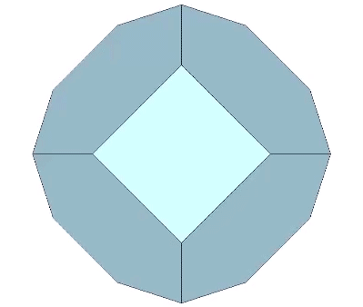
The tetrakaidecahedron that combines with the pyritohedron to fill all space is a 14-sided polyhedron consisting of two elongated hexagonal faces and two sets of pentagonal faces: four matching the faces of the pyritohedron, and eight elongated pentagons.
Lines drawn from the base to peak of the eight elongated pentagon faces, and from the line’s endpoints to the center of the tetrakaidecahedron, form equilateral triangles whose edge lengths in the Weaire-Phelan matrix correspond to the diameter of the nuclear spheres isolated by the pyritohedra.
Lines drawn from the base to the peak of the eight elongated pentagon faces of the tetrakaidechedron (clear blue), and from the line’s endpoints the center, form equilateral triangles whose edge lengths in the Weaire-Phelan matrix correspond to the diameter of the nuclear spheres isolated by the pyritohedra (clear gray).
The appearance of eight equilateral triangles in both the pyritohedron and the tetrakaidecahedron suggests the possibility of a jitterbug-like transformation from one to the other. Their edge lengths, however, differ. The edge length of the eight equilateral triangles in the pyritohedron is approximately 1.091135 times the edge length of those in the tetrakaidecahedron.
Both the tetrakaidecahedron (left) and the pyritohedron (right) disclose eight equilateral triangles, suggesting the possibility of jitterbug-like transformation whereby one transforms into the other. Their respective lengths, however, differ by a factor of 1.091135.
Connecting the unit-length radials of adjacent tetrakaidecahedra forms shells around the nuclei in the shape of Kelvin’s truncated octahedron.
Wireframe the Weaire-Phelan matrix, with 14 tetrakaidecahedra surrounding a pyritohedron and nucleus. Connecting the unit-length radials of adjacent tetrakaidecahedra forms a Kelvin shell around the nucleus.
If we align the unit vectors of the Weaire-Phelan matrix with the isotropic vector matrix, the pyritohedra enclose spaces rather than spheres. If we align them with the distribution of nuclei, the Weaire-Phelan matrix is 180° out of phase with the isotropic vector matrix. This phase difference suggests an energetic relationship between the two matrices that may provide insight into the jitterbug transformation, and its oscillations between spheres and spaces.
The pyritohedron, and the tetrakaidecahedra paired with its mirror image, both align with the The Seven Axes of Symmetry.
Paired tetrakaidecahedra (left) and pyritohedron (right) aligned to the seven axes of symmetry.