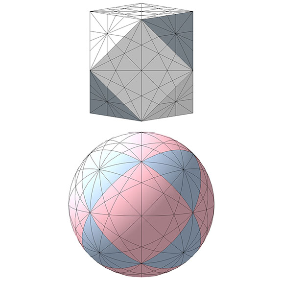
The figure below illustrates the full set of great circles in the context of the vector equilibrium (VE), both the planar VE (top), and spherical VE (bottom). Note that twelve great circles converge, cross, or are deflected at each of the twelve vertices, and at the centers of each triangular face.
The 25 great circles of the vector equilibrium (VE)
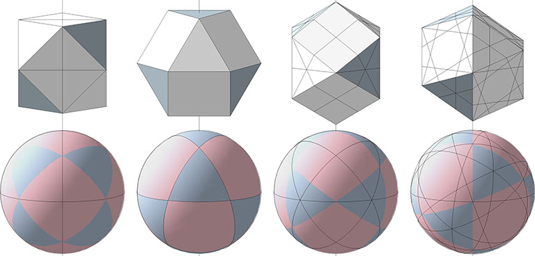
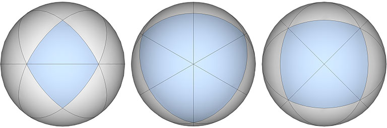
The 25 great circles are divided into four sets according to their spin axes. Axes running through opposite square faces generate the set of 3 great circles. Axes running through the centers of opposite triangular faces generate the set of 4 great circles. Axes running through diametrically opposing vertices generate the set of 6 great circles. And axes running through the midpoints of diametrically opposing edges generate the set of 12 great circles.
Left to right: Set of 3 great circles on axes through opposing square faces; Set of 4 great circles on axes running through opposing triangular faces; Set of 6 great circles on axes running through opposing vertices; Set of 12 great circles with axes running through opposing edges.
3 Great Circles
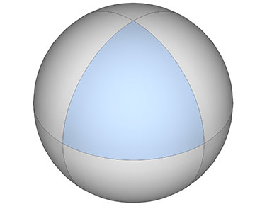
The set of 3 great circles discloses the spherical octahedron.
The spherical octahedron disclosed from the set 3 great circles, with one face highlighted.
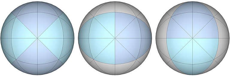
4 Great Circles
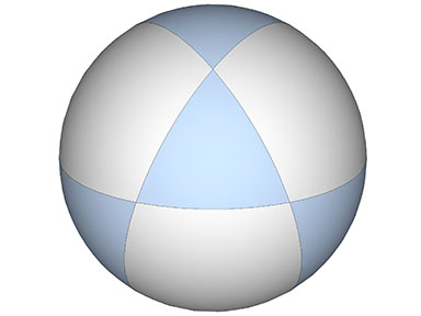
The set of 4 great circles discloses the spherical vector equilibrium (VE).
The spherical VE disclosed from the set of 4 great circles, with its triangular faces highlighted.
6 Great Circles
The six great circles disclose the spherical rhombic dodecahedron, the spherical tetrahedron (both positive and negative), and the spherical cube.
The set of 6 great circles disclosing, left to right: the spherical rhombic dodecahedron; the spherical tetrahedron, and; the spherical cube, each with one face highlighted.
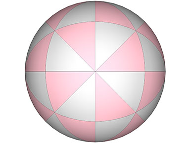
The six great circles complement the three great circles to disclose three additional octahedra.
The sets of 3 and 6 great circles disclose three additional spherical octahedron.
The sets of 3 and 6 great circles of the VE disclose the 48 basic equilibrium LCD triangles.
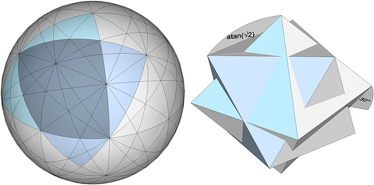
12 Great Circles
The twelve great circles of VE do not appear to disclose, by themselves, any of the regular polyhedra. However, in combination with the 4 and 6 great circle sets, the 12 great circles do disclose an alternate spherical regular octahedron that is curiously askew from the others, rotated 30° on the z axis, and atan(√2) on the y axis.
The 4, 6, and 12 great circles of the VE each contribute one edge to disclose a spherical octahedron whose axes are curiously skewed from all the other polyhedra the 25 great circles of the VE disclose.
“The closest-packed symmetry of uniradius spheres is the mathematical limit case that inadvertently captures all the previously unidentifiable otherness of Universe whose inscrutability we call space. The closest-packed symmetry of uniradius spheres permits the symmetrically discrete differentiation into the individually isolated domains as sensorially comprehensible concave octahedra and concave vector equilibria, which exactly and complementingly intersperse eternally the convex “individualizable phase” of comprehensibility as closest-packed spheres and their exact, individually proportioned, concave-in-betweenness domains as both closest packed around a nuclear uniradius sphere or as closest packed around a nucleus-free prime volume domain.” —R. Buckminster Fuller, Synergetics, 1006.12
Spaces, like spheres, have surfaces. The interstitial model of the isotropic vector matrix (IVM) makes evident that it is the sphere’s surfaces (both its convex and its concave surfaces) that matter. Electric charge is carried on the surface of the conductor. Molecular biology is all about the lock and key system of protein surfaces and shapes. The surface of the “space” in the isotropic vector matrix is a continuity broken only be the seams at the interface of the concave “spaces” and “interstices” (see below). These seams align with the four great circles of the vector equilibrium (VE), and describe the most efficient paths between the points of contact with adjacent spheres. See also: Anatomy of a Sphere.
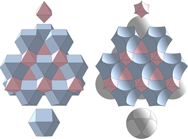
The figure below shows the exact correlation between two models of the isotropic vector matrix, a correspondence that Fuller attempted to describe in the excerpt I’ve quoted above.
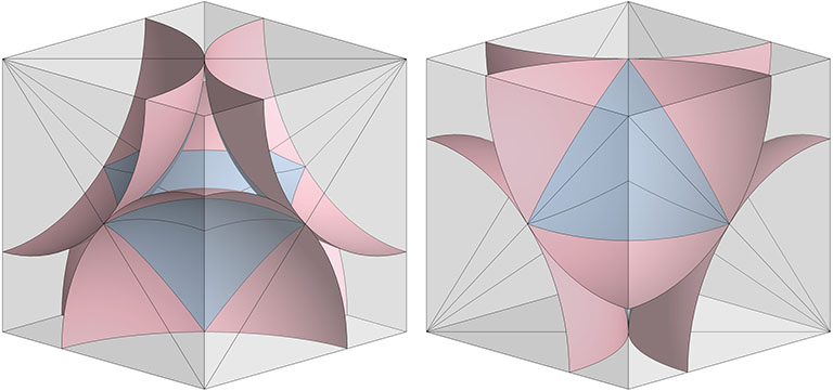
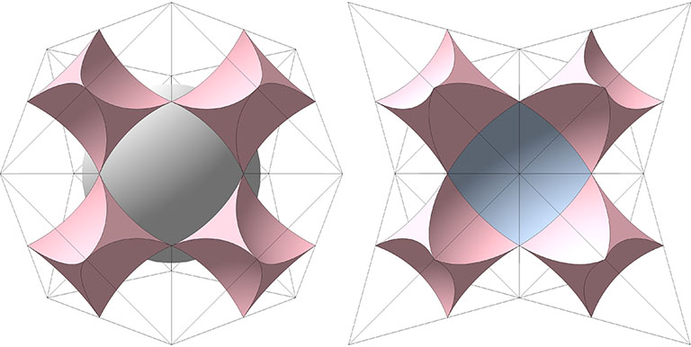
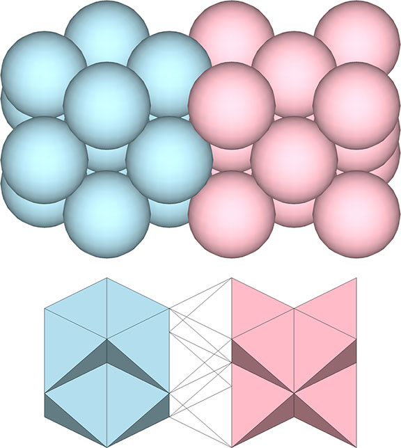
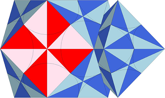
Space Filling of Octahedron and Vector Equilibrium: The packing of concave octahedra, concave vector equilibria, and spherical vector equilibria corresponds exactly to the space filling of planar octahedra and planar vector equilibria. Exactly half of the planar vector equilibria become convex; the other half and all of the planar octahedra become concave.
Though the VEs (blue) and octahedra (pink) on the left align with the spaces (blue) and interstices (pink) on the right, close inspection of the above models reveals a key difference. The model on the left does not distinguish between spheres and spaces. While on the right the difference is obvious, on the left both spheres and spaces are represented by identical VEs. The ambiguity is apt: In the isotropic vector matrix, there is a one-to-one identity between the spheres and spaces; one is simply the other turned inside out.
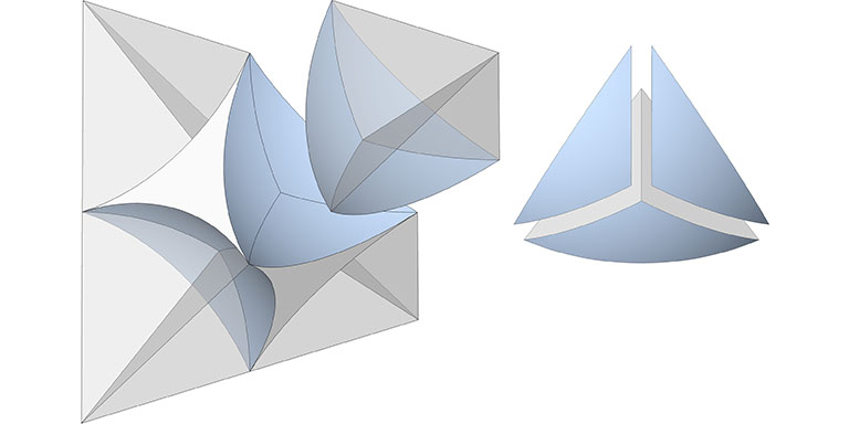
The model on the right is what I’m calling the interstitial model of the isotropic vector matrix. It consists of concave vector equilibrium (VE) spaces and concave octahedron interstices. The concave VE is the shape of the void at the center of six close-packed spheres defining the octahedron. The concave octahedron is the shape of the void at the center of four close-packed spheres defining the tetrahedron.
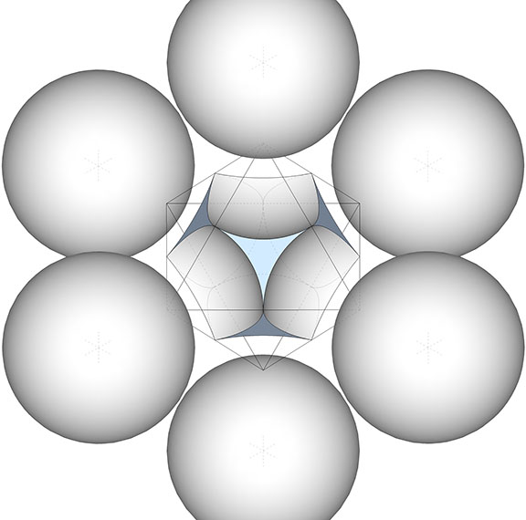
Concave VE (“space”)
Because it occupies the space in the isotropic vector matrix that is replaced by a sphere in the jitterbug transformation, I reserve the term “space” for the concave VE at the common center of the six close-packed spheres of the regular octahedron.
The void at the center of the six close-packed spheres centered on the vertices of the regular octahedron has the shape of a concave vector equilibrium (VE). In the jitterbug transformation, this “space” is turned inside-out to define the spherical VE or “sphere.”
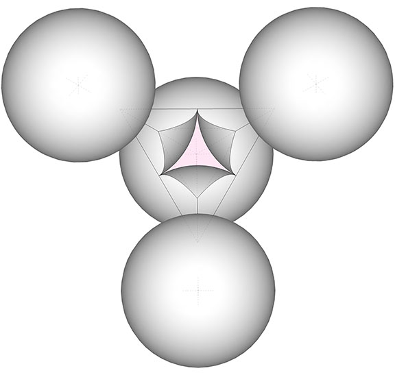
Concave Octahedron (“interstice”)
The void at the center of four close-packed spheres has the shape of a concave octahedron which I call the “interstice” to distinguish it from the “space” referred to above. The interstices maintain both their shape and position during the jitterbug transformation, while their 90° rotations articulate the sphere-to-space oscillations described below.
The void at the center of the four spheres centered on the vertices of the regular tetrahedron has the shape of a concave octahedron. These “interstices” are rotated 90° to alternately define the spheres and spaces that exchange places in the jitterbug transformation.
Spherical Domains
The polyhedra of the isotropic vector matrix divide the spheres into rational sections which, when added together, constitute the polyhedron’s spherical domain. Fuller thought this rationality was sufficient to eliminate pi (π) from his geometry. He’d already shown that the volumes of most polyhedra were rational if instead of the cube we used the regular tetrahedron as the unit volume. And if we replaced the irrational volume of the sphere with the rational sections carved from the rational polyhedra, pi was irrelevant.
Rhombic Dodecahedron
144 quanta modules
1 spherical domain
Vector Equilibrium (VE)
480 quanta modules
3.40 spherical domains
Cube
72 quanta modules
1/2 spherical domain
Octahedron
96 quanta modules
3/5 spherical domain
Tetrahedron
24 quanta modules
1/5 spherical domain
Octahedron
The six spheres at the vertices of the octahedron define the concave vector equilibrium space at its center. The planar facets of each vertex carve a 1/10 section from its sphere. The 1/10 section is further subdivided to form the four 1/40 sections used in the spherical domain calculations. The total spherical domain of the planar octahedron is 3/5.
The planar octahedron cuts 1/10 sections from each of its six spheres, for a total spherical domain of 3/5. Each of these 1/10 sections is further subdivided into four 1/40 sections which are used to calculate the spherical domains of the remaining polyhedra.
Tetrahedron
The four spheres at the vertices of the tetrahedron define the concave octahedron interstice at its center. The planar facets of each vertex carve a 1/20 section from its sphere. The 1/20 section is further divided to form the three 1/60 sections used in the spherical domain calculations. The total spherical domain of the planar tetrahedron is 1/5.
The planar tetrahedron cuts 1/20 sections from each of its four spheres, for a total spherical domain of 1/5. Each of these 1/20 sections is further subdivided into three 1/60 sections which are used to calculate the spherical domains of the remaining polyhedra.
Rhombic Dodecahedron
There are two rhombic dodecahedra in the isotropic vector matrix—one with a space at its center, and one with a sphere. For the rhombic dodecahedron with a space at its center, each of the six acute vertices define the center of a sphere from which the planar facets of each carve a 1/6 section. Both of the planar rhombic dodecahedra contain precisely one spherical domain.
Note that one is made from the other by reversing the 1/6 sections so that their peaks point either inward to define the sphere, or outward to define the space.
The planar rhombic dodecahedron on the left cuts 1/6 sections from each of the six spheres centered on its six acute vertices, for a total spherical domain of 1, the same spherical domain of the rhombic dodecahedron on the right, where the 1/6 sections have been rotated 180° so that their convex faces are pointing outward.
Cube
There are two cubes in the isotropic vector matrix, one a 90° rotation of the other. Their rotation comprises the jitterbug transformation and the exchange between spheres and spaces. Four of its eight vertices each define the center of a sphere from which the planar facets of each carve a 1/8 section. The planar cube contains precisely 1/2 spherical domain.
The planar cube carves a 1/8 section from the spheres centered on four of its eight vertices, for a total spherical domain of 1/2. The cube on the right is a 90° rotation of the cube on the left. This rotation accounts for the sphere-to-space oscillations of the isotropic vector matrix in the jitterbug transformation.
Vector Equilibrium (VE)
The twelve vertices of the VE each define the center of a sphere from which the planar facets carve a 1/5 section. These plus the nuclear sphere add to a total of 3.4 spherical domains.
The planar vector equilibrium (VE) carves 1/5 sections from each of the twelve spheres centered on its vertices. These plus the nuclear sphere total add to 3.4 spherical domains.
Ratio of Spheres to Spaces in the Isotropic Vector Matrix
While the sphere-to-space ratio differs for the polyhedra, when the isotropic vector matrix is considered as a whole the ratio approaches that of the rhombic dodecahedron; rhombic dodecahedra close pack exactly as spheres close pack, and the rhombic dodecahedron constitutes one spherical domain.
The volume of the unit-diameter sphere is π√2 tetrahedra and the volume of the rhombic dodecahedron which contains that sphere is six unit tetrahedra. So, the sphere-to-space ratio is (π√2)/(6 – π√2), or ≈ 2.853275. Fuller wanted this number to be rational. It is not.
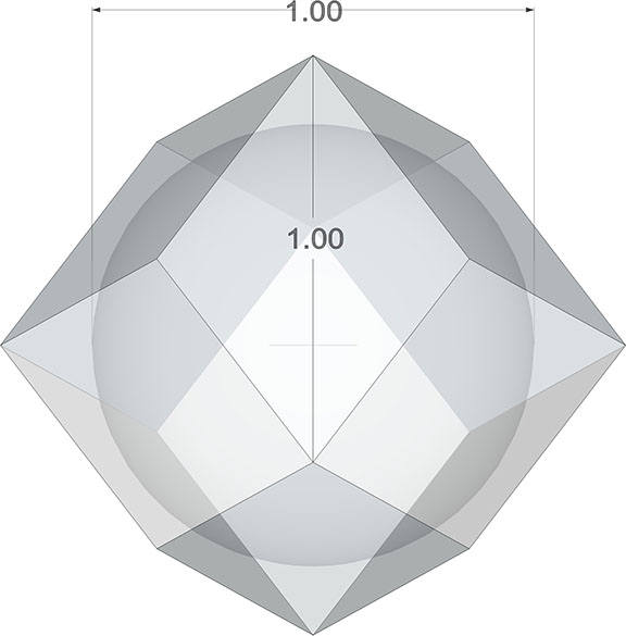
The domain of the radially close-packed unit-diameter sphere is a rhombic dodecahedron whose in-sphere radius and long face diagonal are of unit length, and whose tetrahedral volume is exactly 6.
Sphere-to-Space and Space-to-Sphere Oscillation of the Jitterbug
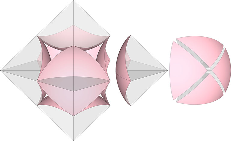
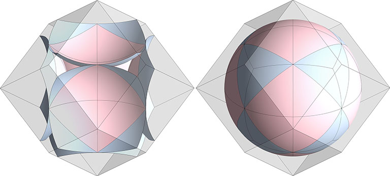
The interstitial model provides the most literal interpretation of the space-to-sphere oscillations of the jitterbug. The tetrahedron’s polarity reversal is accomplished by a 90° rotation of the concave octahedron interstices which alternately disclose the nuclear sphere, on the left in the illustration below, and the nuclear space, on the right:
The concave octahedron interstices are rotated 90° to alternately disclose the nuclear sphere at the center of the vector equilibrium (left), and the nuclear space at the center of the octahedron (right).
The 90° rotation of the concave octahedra interstices at the centers of positive and negative tetrahedra account for the sphere-space oscillations of the jitterbug transformation.
Fuller’s four primary models of the isotropic vector matrix—as vectors, as spheres, as the interstices between spheres, and as A and B quanta modules, are as distinct as they are inseparable. Each serves different purposes in Fuller’s geometry, and the terms used for one model are not necessarily synonymous with the same terms applied to another.
For example, the regular tetrahedron and the regular octahedron of the vector model each complement the other to fill all-space. In the sphere model, the tetrahedron is comprised of four spheres that define the domains of the tetrahedron’s four vertices in the vector model, and likewise, the octahedron is comprised of six spheres defining the domains of its vertices. These tetrahedra and octahedra do individually close-pack in the sphere model.
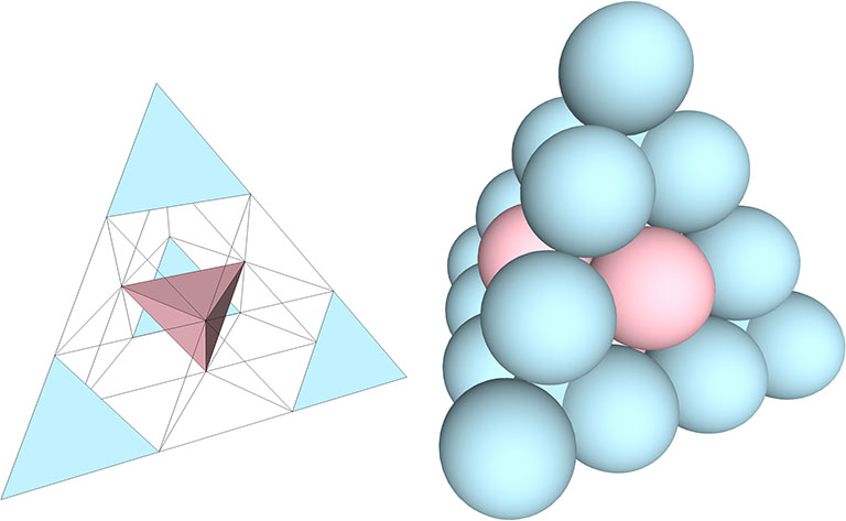
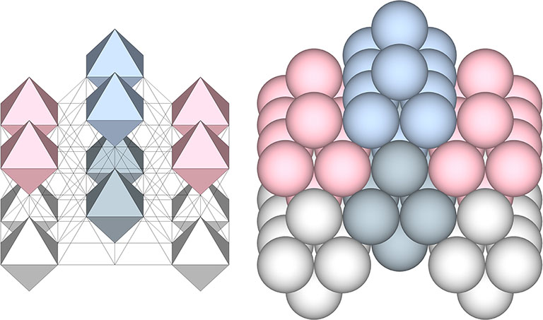
In the first illustration below, five 4-sphere tetrahedra (four positive and one negative) have been stacked to form the F3 tetrahedron on the right. On the left is the vector model of the same F3 tetrahedron. You’ll note that the domains of all the vertices are occupied by the four-sphere tetrahedra in the sphere model, even though space remains (in the shape of edge-bonded octahedra) between the tetrahedra in the vector model.
4-sphere tetrahedra (right) close-pack to occupy all the vertices of the isotropic vector matrix (left).
Similarly, six-sphere octahedra (right) close-pack to occupy the domains of all the vertices in the vector model (left):
6-sphere octahedra (right) close-pack to occupy all the vertices of the isotropic vector matrix (left).
And, 13-sphere VEs and 14-sphere cubes (top) close-pack in combination to occupy the domains of every vertex in the vector model (bottom):
13-sphere vector equilibria (VEs) and cubes (top) close-pack to occupy all the vertices of the isotropic vector matrix (bottom).
Incidentally, this last illustration is also a model of the jitterbug transformation. See: Jitterbug.
Another way of thinking about the different models of the isostropic vector matrix is to imagine the spheres model as squeezing the vector model’s close-packed tetrahedra and octahedra into the concave VEs and concave octahedra of the interstitial model. (See Spheres and Spaces, and Spaces and Spheres (Redux).)
A curious mathematical coincidence that I think is worth noting is that the edge length of the tetrahedron in which a unit octahedron or unit icosahedron is inscribed is numerically equivalent to the units of volume, in tetrahedra, provided by each of the inscribed polyhedron’s structural quanta. (For more information on calculating volumes in tetrahedra, see Areas and Volumes in Triangles and Tetrahedra.)
A structural quantum is defined by the six edges of the minimum structural system. The six edges of the tetrahedron comprise one structural quantum, the twelve edges of the octahedron comprise two structural quanta, and the thirty edges of the icosahedron comprise five structural quanta.
In the regular tetrahedron, one structural quantum encloses 1 unit of volume. In the regular octahedron, one structural quantum encloses 2 units of volume. And, in the regular icosahedron, one structural quantum encloses Φ²√2 units of volume (where Φ is the golden ratio: (√5+1)/2).
If these unit polyhedra (i.e., all edges are of unit length) are inscribed within a regular tetrahedron, the edge length of the enclosing tetrahedron is numerically equivalent to the volume enclosed by each structural quantum of the inscribed polyhedron.
The edge length of the tetrahedron in which a unit octahedron or unit icosahedron is inscribed is numerically equivalent to the units of volume provided by each of the inscribed polyhedron’s structural quanta
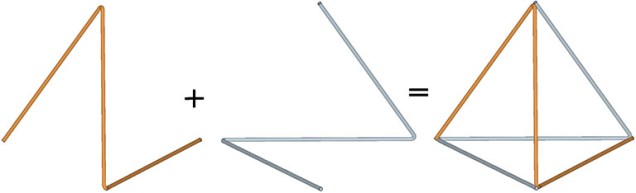
Fuller’s “structural quanta” are related to the idea that all the structural polyhedra can be thought of as self-interfering wave patterns. Each cycle of the wave consists of the three vectors of an open ended triangle. The tetrahedron, for example, consists of two open-ended triangles, one clockwise and one counter-clockwise, as in the following illustration:
The tetrahedron as a self-interfering wave pattern. The waves are represented here as two open-ended triangles (left), one clockwise and one counter-clockwise, which combine to form the four triangles of the tetrahedron (right).
I’ve used the equations described in this topic to calculate the strut and tendon lengths of the tensegrity sphere models I describe in Model Making. They are slightly modified from those published by Hugh Kenner in his book, Geodesic Math and How To Use It (1976, 2003). See also: Tensegrity.
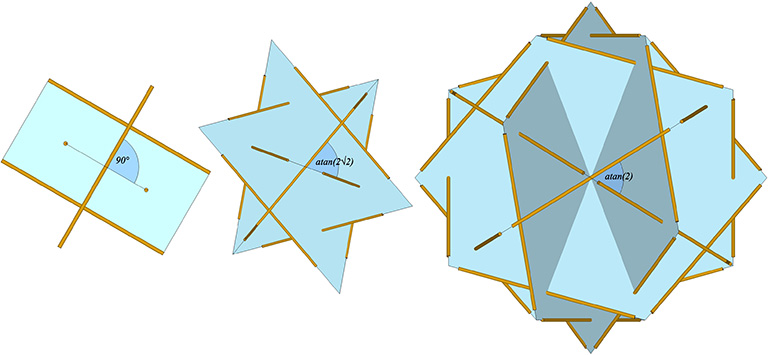
After some rather clever reasoning, Kenner concluded that all of the dimensions of the tensegrity spheres could be derived from just two quantities: the number of sides (n) in their great circle (or lesser circle) planes, and the angle (µ) at which they cross. The following illustration shows the three primary tensegrity spheres, i.e., the spherical phases of the tensegrity tetrahedron, octahedron, and icosahedron:
the six-strut tensegrity sphere with three great circles planes of two struts (n=2), each crossing at µ=90°;
the twelve-strut tensegrity sphere with four great-circle planes of three struts (n=3), each crossing at µ=atan(2√2) ≈ 70.530°; and,
the thirty-strut tensegrity sphere with six great circle planes of five struts (n=5), each crossing at µ=atan(2) ≈ 60.435°.
The great circle planes of the six-, twelve-, and thirty-strut tensegrity spheres, and the angles at which they intersect
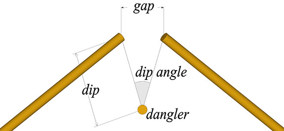
The intersection of the great-circle and lesser-circle planes can be broken down to two struts and a dangler, as in the following illustration.
The gap, dip, and dip angle are parameters used in the calculations for tensegrity structures.
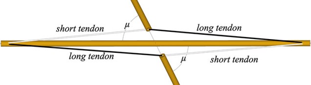
The dangler strut’s great circle crosses the great circle of the other two struts at an angle, µ. If this angle is less than 90° (as is the case for all but the six-strut tensegrity sphere), the tension elements will consist of a long and a short tendon, as shown in the following illustration.
Two struts of a great circle plane crossing the midpoint of a dangler at angle, µ, with the long and short tendons connecting their endpoints.
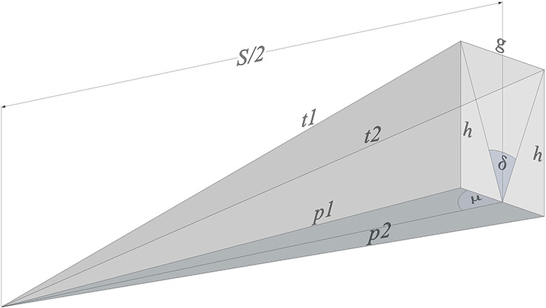
The next illustration shows the relationships between all the parameters that go into calculating the circumsphere radius, strut length, and tendon lengths of the tensegrity spheres:
S = strut length;
r = the circumsphere radius, from sphere center to each of the strut endpoints;
dangler = the strut bisected by the great circle plane of two struts;
μ = the angle the great circle plane of the dangler makes with the great circle plane of the two struts;
d = dip, i.e., the distance between each strut’s endpoint and the midpoint of its dangler;
δ = the dip angle, i.e., the angle between the dangler’s midpoint and the two strut endpoints;
g = the gap, i.e. the linear distance between the two strut endpoints;
h = the vertical distance between a strut’s endpoint and the horizontal plane of its dangler;
t1 and t2 = the length of the short and long tendons, respectively;
p1 and p2 = the base of the right angle made with h, and with t1 or t2 as its hypotenuse, respectively.
Parameters and equations used to calculate the tendon lengths (t1 and t2) of the three primary tensegrity spheres.
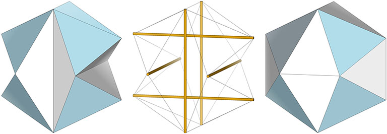
The Jessen Orthogonal Icosahedron (center) constructed from two overlapping VEs (left and right). Click on image to open animation in new tab.
This is halfway between the nuclear sphere at the center of the VE and the space at the centers of its constituent octahedra. The location is apt, as the Jessen marks the halfway point in the jitterbug transformation between the VE and octahedron, i.e., between spheres and spaces.
The Jessen Orthogonal Icosahedron (blue) occupies a position in the isotropic vector matrix diametrically halfway between the spheres and spaces at the centers of VEs and octahedra in the isotropic vector matrix.
The Jessen has a rational tetrahedral volume. If we attempt to isolate the space it occupies in the quanta module construction of the isotropic matrix, we discover that it can almost, but not entirely be modeled in A and B quanta modules.
The position of the Jessen Orthogonal Icosahedron in the quanta module construction of the isotropic matrix. Click on lower image to open animation in new tab.
At the center of the quanta module construction of the Jessen is the eight-Mite coupler that joins spheres with spaces.
An eight-Mite coupler lies the center of the Jessen Orthogonal Icosahedron, shown here as the six-strut tensegrity sphere whose struts and tendons define the Jessen’s edges. Click on image to view animation in new tab.
Note that the coupler is polarized and seems to point, forwards and backwards, along the vector of its displacement between the VE and octahedron, i.e. from the sphere in the direction of its adjoining space (or vice versa). The only other polyhedron whose quanta module construction is similarly polarized is the cube. The orientation of the cube in the quanta module construction of the isotropic vector matrix determines the polarity of the tetrahedron, and the six-strut tensegrity that defines the Jessen is the spherical phase of the tensegrity tetrahedron, the wave function, if you will, that collapses into either a positive or negative tetrahedron. (See also: Dual Nature of the Tetrahedron.)
“Transformation of Six-Strut Tensegrity Structures: A six-strut tensegrity tetrahedron can be transformed by changing the distribution and relative lengths of its tension members to the six-strut icosahedron [Jessen Orthogonal Icosahedron]. A theoretical three-way coordinate expansion can be envisioned with three parallel pairs of constant-length struts in which a stretching of tension members is permitted as the struts move outwardly from a common center. Starting with a six-strut octahedron, the structure expands outwardly going through the icosahedron phase to the vector-equilibrium phase. When the structure expands beyond the vector equilibrium, the six struts […] lose their structural function (assuming the original distribution of tension and compression members remains unchanged). As the tension members become substantially longer than the struts, the struts tend to approach relative zero and the overall shape of the structure approaches a super octahedron.” —R. Buckminster Fuller, Synergetics, 725.02
Fuller recognized that the six-strut tensegrity structure (which he often referred to as the “tensegrity icosahedron”) and the polyhedron that we are here calling the Jessen Orthogonal Icosahedron, was actually a transformation of the tensegrity Tetrahedron. As I’ve said elsewhere, all that can be reasonably called “structure” in the universe is, fundamentally, a self-supporting integrated system of continuous tension and discontinuous compression that Fuller termed, Tensegrity.
The Jessen Orthogonal Icosahedron represents the spherical, or what I’m calling the “tensor equilibrium” phase, of the tetrahedron. It occurs at the halfway point in the transformation by which the tetrahedron reverses itself, from its positive (clockwise) to its negative (counter-clockwise) state and vice versa. (See illustration below.) The tetrahedron may be unique in this ability. See Dual Nature of the Tetrahedron.
The 6-strut tensegrity is the spherical phase of the tensegrity tetrahedron, seen here transforming to either a positive or a negative tetrahedron.
Approximately midway between its vector-equilibrium phases, the jitterbug describes the regular icosahedron. The collapsing VEs and expanding octahedra, however, do not simultaneously describe the regular icosahedron. The common shape, precisely midway between the transformation from one to the other, is actually the shape of the six-strut tensegrity sphere. This is the “tensor equilibrium” phase of the isotropic vector matrix, in contrast to the more familiar “vector equilibrium” phase.
Precisely midway through the jitterbug transformation, the isotropic vector matrix reaches tensor equilibrium; the contracting VEs and the expanding octahedra oscillate between their vector equilibrium phases and simultaneously describe the shape of the 6-strut tensegrity sphere, or “Jessen Orthogonal Icosahedron.”
Fuller neglected to give the shape a name, perhaps failing to appreciate its full significance. Other mathematicians, namely Borge Jessen, have taken credit for its “discovery,” and Wikipedia affirms its identity as the Jessen Orthogonal Icosahedron.
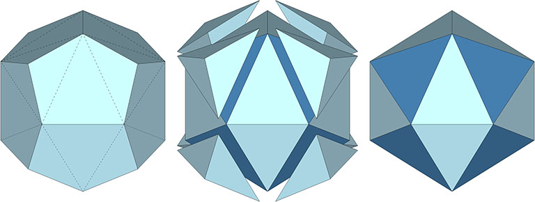
The Jessen Orthogonal Icosahedron (left) describes the shape of the 6-strut tensegrity sphere (center); its concave faces may be replaced with convex faces by rotating their shared base vector 90° and connecting the vertices of their short diagonal (right).
Tensor equilibrium is made intuitively obvious with a physical model of the six-strut tensegrity sphere constructed of rigid struts and elastic tendons.** By pulling apart or squeezing together any one pair of opposing struts, the whole structure symmetrically expands and contracts, i.e. “jitterbugs” between the vector equilibrium states of the VE, at maximum separation, and the octahedron, when each strut pair is bunched together. Between these two maximally stressed states is the Jessen orthogonal icosahedron, or six-strut tensegrity sphere, the unstressed state about which the tensegrity oscillates.
Pulling apart or squeezing together any one pair of opposing struts transforms the six-strut tensegrity causes the others to likewise expand and contract, i.e., to “jitterbug” between the VE and Octahedron.
The tensor equilibrium state is also physically and convincingly demonstrated with the models in the following illustration.
Physical models demonstrating tensor equilibrium include, left to right: the 6-strut tensegrity with the tension web replaced with elastic slings; elastic loops stretched between a cubic scaffold with frictionless rings; the conventional model of the six-strut tensegrity with its continuous tension web; and the Jessen Orthogonal Icosahedron on the far right.
The model on the left is the six-strut tensegrity sphere with its continuous web of tension replaced by rubber-band slings. Second from left is a model built with elastic loops stretched between the edges of a cubic scaffold with frictionless rings. Second from right is the conventional model of the six-strut tensegrity sphere. All of these models slip naturally into their equilibrium state which conforms precisely to the shape of the Jessen Orthogonal Icosahedron on the far right.
** For detailed instructions for constructing these and other models relevant to Fuller’s geometry, see the page, Model Making, on this web site.
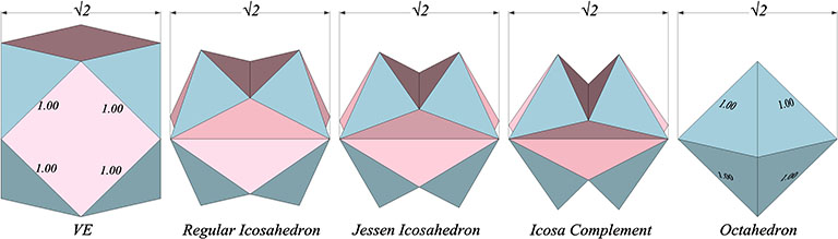
If the long edges of the Jessen’s concave faces are imagined to be the struts of the the six-strut tensegrity sphere, their length would be the square root of two (√2) — the same as the diagonal of the square face of the unit-edge VE and the circumsphere diameter of the unit-edge octahedron. Given a strut length of √2, the Jessen has a rational tetrahedral volume. If the struts are taken to be of unit length, the Jessen has a rational cubic volume.
The phases of the jitterbug transformation with the strut length (long edge of the concave icosahedra) held constant at √2.
If the strut length (d) is taken to be √2,
the concave Jessen’s tetrahedral volume is exactly 7.5, and;
the convex Jessen’s tetrahedral volume is exactly 10.5.
If the strut length (d) is taken to be of unit length (1.00),
the concave Jessen’s cubic volume is exactly 5/16, and;
the convex Jessens cubic volume is exactly 7/16.
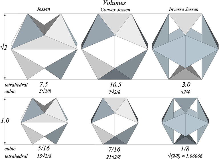
Volumes of the Jessen represented in its concave and convex forms (first and second columns) and as the volumetric difference between the two (right column). Note the tetrahedral volumes are rational when the strut length (long concave edge) is held constant at √2, and that the cubic volumes are rational with the strut length (long concave edge) is held constant at unit length.
The polyhedral form of the Jessen can be represented as six irregular tetrahedra occupying the Jessen’s concavities (right column in the above illustration). With the length of their long edge (strut) equal to √2 their combined tetrahedral volume is 3, the same tetrahedral volume as the unit-diagonal cube. With a unit strut length (d=1), their cubic volume is 1/8, and their tetrahedral volume is, significantly, exactly the value of Fuller’s “Synergetics Conversion Constant,” √(9/8), approximately 1.066066. See Pi and the Synergetics Constants.
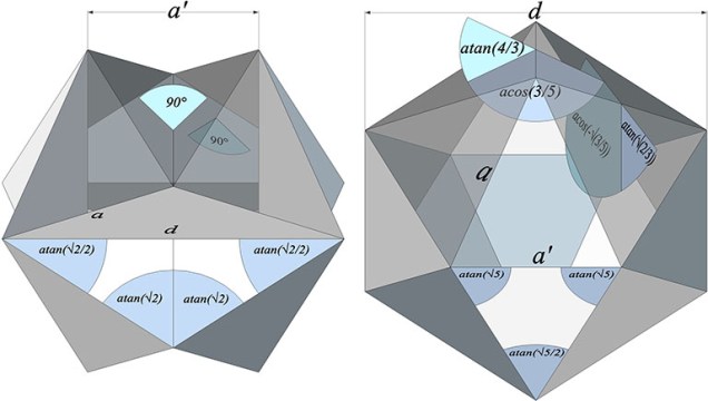
“Orthogonal” refers to the Jessen’s definitive concave form in which its dihedral angles are all 90°; that is, all of the Jessen Orthogonal Icosahedron’s faces meet at right angles. In the Jessen’s convex form, the cosine of one dihedral is the second root of the other: acos(-3/5), and; acos(-√(3/5)), which seems somehow significant.
Dihedral and surface angles of the concave (left) and convex (right) Jessen.
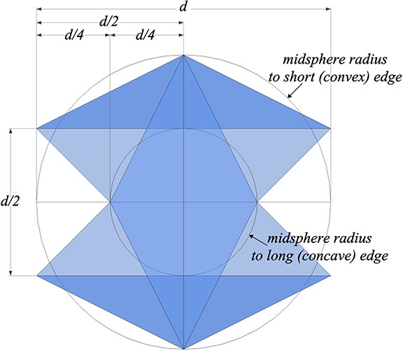
The smallest radius of the Jessen is the midsphere radius to its long (concave) edge, and is exactly 1/4 the strut length, or d/4. In its convex form, the midsphere radius to its short (convex) edge is now doubled to d/2. This may be made more clear in the following illustration:
The midsphere radius from the Jessen’s center of volume to the short edge of its concave faces is exactly half the midsphere radius to the long edge of its concave faces, or 1/2 and 1/4 the strut length (d) of the 6-strut tensegrity sphere.
All the other radii are irrational with respect to both the edge length (a) and strut length (d).
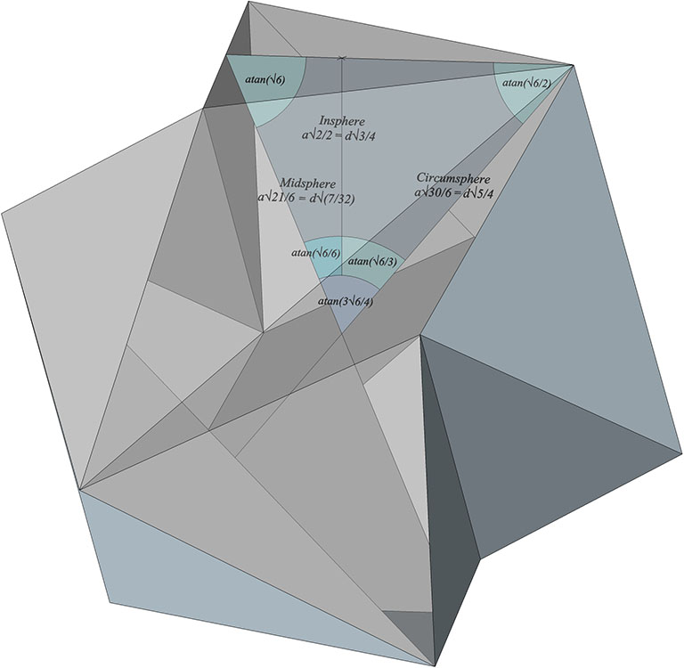
The Jessen’s circumsphere radius and the midsphere radius to its edge (a) forms a triangle of atan(√6), atan(√6/2), and atan(3√6/4). The insphere radius divides the latter angle into atan(√6/6) and atan(√6/3).
Insphere, midsphere, and circumsphere radii of the Jessen to its equilateral triangular face.
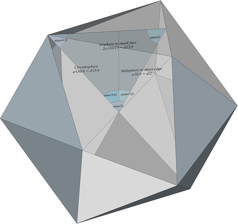
The Jessen’s circumsphere radius and the midsphere radius to its short (convex) edge (a’) forms an isosceles with rational trigonometry: atan(2), atan(4/3), and atan(2). The insphere radius divides the latter angle into atan(1/2) and atan(3/4).
Insphere, midsphere, and circumsphere radii of the Jessen to its isosceles triangle (convex) face.
The dimensions of the Jessen relative to its tendon (aka edge) length (a), and its strut (aka long edge) length (d) are provided below:
a = edge (tendon) length a’ = short edge length of convex face d = long edge (strut) length d = a × 2√6/3 a = d × √6/4 a’ = a × √6/3 = d × 1/2 Insphere radius = a × √2/2 = d × √3/4 Insphere radius to small face = a × 2√30/15 = d × √5/5 Midsphere radius = a × √21/6 = d × √14/8 Midsphere radius to short edge of convex face = a × √6/3 = d × 1/2 Midsphere radius to long edge of concave face = a × √6/6 = d × 1/4 Circumsphere radius = a × √30/6 = d × √5/4 Face angles (convex): atan(√5/2), atan(√5/2), atan(√5) Face angles (concave): atan(√2/2), atan(√2/2), acos(-1/3) Dihedral angles (convex form): acos(-3/5); acos(-√(3/5)) Dihedral angles: all 90° Cubic Volume (concave form) = a³ × 5√6/9 = d³ × 5/16 Tetrahedral Volume (concave form) = a³× 20√3/3 = d³ × 15√2/8 Cubic Volume (convex form) = a³ × 7√6/9 = d³ × 7/16 Tetrahedral Volume (convex form) = a³× 28√3/3 = d³ × 21√2/8
As noted earlier, the Jessen has rational cubic volume of 5/16 when the strut length (long edge) is of unit length; the Jessen has a rational tetrahedral volume of 7.5 when the strut length (long edge) preserves its length at vector equilibrium, i.e. √2. This is a gratifying result, and reinforces my view that the Jessen models an equilibrium phase of the isotropic vector matrix.
The Jessen icosahedron is a truncation of the pyritohedron.
Truncating the vertices of the pyritohedron (left) results in the convex form of the Jessen (right).
The struts (or long edges of the concave faces) of the Jessen align with the tetrakaidecahedra of the Weaire-Phelan matrix. (See: Tetrakaidecahedron and Pyritohedron.)
The struts of the 6-strut tensegrity align with the orthogonal distribution of tetrakaidecahedra in the Weaire-Phelan matrix.
These and other clues seem to point to a relationship between the tetrakaidecahedron-pyritohedron matrix (aka, the Weaire-Phelan structure) and tensor equilibrium, in addition to the relationship between the close packing of the voids in foam matrices with the close-packing of spheres and the distribution of nuclei in the isotropic vector matrix.
“The icosahedron positioned in the octahedron describes the S Quanta Modules. […] As skewed off the octa-icosa matrix, they are the volumetric counterpart of the A and B Quanta Modules as manifest in the nonnucleated icosahedron. They also correspond to the 1/120th tetrahedron of which the triacontahedron is composed.” —R. Buckminster Fuller, Synergetics, 988.110
The S quanta module is documented in Synergetics, but it doesn’t seem to have led Fuller anywhere. It was, I think, an attempt to rationalize the volume of the icosahedron, or, at the very least, to calculate the volume of the icosahedron that is inscribed inside the regular octahedron. See Icosahedron Inside Octahedron. Fuller’s operational method is provided here, along with my own calculations which, it should be noted, don’t always agree with Fuller’s.
With a regular icosahedron placed inside a regular octahedron with unit-length edges, the space not occupied by the icosahedron is subdivided into 24 irregular tetrahedron, 12 positive and 12 negative. These are the S quanta modules.
With a regular icosahedron placed inside a regular octahedron, the space not occupied by the icosahedron is subdivided into 24 irregular tetrahedra, 12 positive and 12 negative. These are the S Quanta Modules.
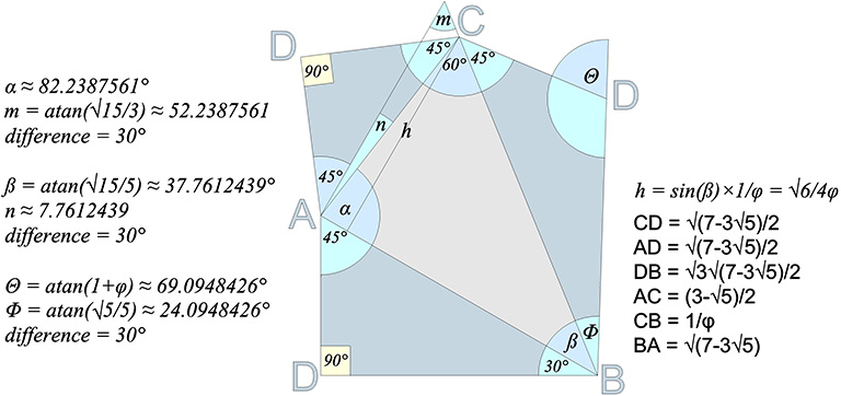
With the edge of the octahedron, a, taken as unity, the six edges of the S quanta module have the following lengths:
AC = a(3-√5)/2; CB = a/φ; AC+CB = a = 1 BA = a√(7-3√5); AD = a√(7-3√5)/2; BD = a√3×√(7-3√5)/2, and; CD = a√(7-3√5)/2
With the edge of the icosahedron, d, taken as unity, the six edges of the S quanta module have the following lengths:
AC = d√3/2 CB ≈ d×0.9045085 BA = d = 1 AD = d/2 BD = d√3/2 CD = d/2
A (45°,α, 45°); B (30°, ß, Φ); C (45°,60°,45°), and; D (90°, 90°, (180°- Θ))
Note that the difference of 90° and α (i.e. 90°−82.2387561°) is 7.7612439°, or arctan(√(3/5))-30°. (See angle n in figure below.) This is the same angle that separates the icosahedron phases of the jitterbug.
The S quanta module unfolded from the external face (light gray triangle).
To calculate the volume of the S quanta module, we first find the area of its external face which will be taken as the S module’s base.
Base of external face of S module = BA = a√(7-3√5) = d 90° height of external face of S module = h = sin(ß) × BC = √6/4 × a/φ ≈ √6/4 × d×0.9045085 60° height of external face of S module = h’ = h × 2√3/3 = a√6/4φ × 2√3/3 = a√2/2φ ≈ √6/4 × d×0.9045085 × 2√3/3 ≈ √2d/2 × 0.9045085 Area of external face of S module (in equilateral triangles) = BA × h’ = a√(7-3√5) × a√2/2φ ≈ a² × 0.2063310 ≈ d × (√2d/2 × 0.9045085) 90° height of S module = AD 60° height of S module = h” = AD × √6/2 Volume of S module (in tetrahedra) = Area of external face × h”
The volume of the A quanta module is 1/24th that of the unit tetrahedron, or ≈ 0.041666, and the volume of the S quanta module is about 1.87415 times that of the A quanta module. Fuller thought the S module’s volume was 1.0820 times that of the A module’s. If we divide the volume of the S quanta module by 2, the volume of the A quanta module is about 1.06715 times that of the halved S quanta module, and that’s as close as I’ve come to Fuller’s figure, which remains a mystery.
The volume of space in the octahedron that is not occupied by the icosahedron is the S module’s volume times 24 ≈ 1.874147087. That leaves a volume of approximately 2.125852913 for the inscribed icosahedron. I haven’t found anything meaningful in these numbers.
Pyritohedra and tetrakaidecahedra close pack to constitute the Weaire-Phelan structure (or Weaire-Phelan “matrix” as I prefer to call it, and, when dimensioned appropriately, align precisely with the distribution of nuclei in the isotropic vector matrix. The unit vector (d in the illustration below) is identical with the unit vector (sphere diameter) of the isotropic vector matrix.
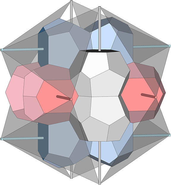
The pyritohedron (right) and the tetrakaidecahedron (left) combine to form the Weaire-Phelan structure (or matrix) and, when dimensioned appropriately, align with the distribution of unique nuclei (red) and shared nuclei (pink) in the isotropic vector matrix.
The pyritohedron and, presumably, the tetrakaidecahedron have identical rational volumes in both cubic and tetrahedral units of measure. For the cubic volume, we take the long edge of the pentagonal face as the unit length (a in the illustrations). For the tetrahedral volume, we take the diameter of the sphere as the unit length (d in the illustrations).
The dimensions of the pyritohedron’s pentagonal face are all related rationally to the length of its long edge, a, which is irrational with respect to d, the diameter of the unit sphere.
When we measure the angles, edge lengths, and radii of the pyritohedron, the numbers do not inspire confidence. It would seem unlikely that so many irrational numbers could possibly result in a rational, whole-number volume. But they do.
a = long edge or base of pentagonal face d = diameter of sphere* d = a × ³√4 × √2/2 a = d × ³(√2/2) = (d√2)/(³√4) = d√2 × ³√(1/4)
*d is identical with the unit vector of the isotropic vector matrix. In the Weaire-Phelan matrix, it aligns with the height vectors connecting the base with the peak of the smaller of the two pentagonal faces of the tetrakaidecahedron, and to the radial vectors connecting the height vector’s endpoints (see illustration below).
The unit vector, d, used in the volume calculations of the pyritohedron (right) is identical with the unit vector in the isotropic vector matrix, i.e. the diameter of the unit sphere. It aligns with the Weaire-Phelan matrix as the radial vectors and face heights in the tetrakaidecahedron (left).
The long edge of the pyritohedron’s pentagonal face, a, (which, when taken as unit length results in a cubic volume for the pyritohedron of 4a³) seems to be related to the diameter of the sphere, d, by ³(√2/2) or about 0.890898718. I don’t have a geometric proof to account for the appearance of this third root, but the number seems to work to at least 7 decimal places in my computer models, and the irrational roots cancel out perfectly in the volume calculations to produce the rational result of 24d³ for the tetrahedral volume.
*It should be possible to construct the pyritohedron from quanta modules, but may involve one or more variants of those quanta modules already described by by Fuller.
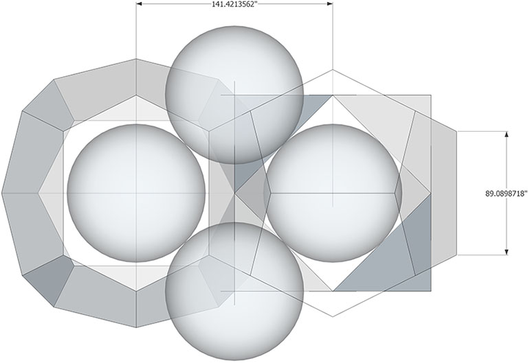
The image below shows my computer model with the calculated dimensions accurate to 7 decimal places.
If the circumsphere radius of the tetrakaidecahedron is of unit length (one sphere diameter), the long edge of the pyritohedron is, to an accuracy of at least seven decimal places, equal to √2׳√(1/4), or about 0.890898718, which produces a rational volume of 24 unit tetrahedra for both the pyritohedron and its complementary tetrakaidecahedron.
Geodesic polyhedra are convex polyhedra consisting of triangles, and include the spherical polyhedra generated by subdividing the faces of a tetrahedron, octahedron, or icosahedron into smaller triangles and projecting their crossings out to the underlying polyhedron’s circumsphere radius. Those based on the icosahedron are related to but not necessarily aligned with the 31 great circles of the icosahedron from which their name seems to have originated. The name “geodesic” refers to Fuller’s early conviction that only a triangular latticework of geodesic lines would serve to distribute local stresses evenly throughout the system he patented under the name “Geodesic Dome” in 1954. As the domes evolved into the systems of mostly partial great circles and lesser circles described here, the term “geodesic polyhedra” preserved the memory of that earlier conviction.
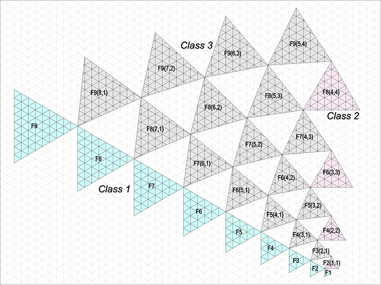
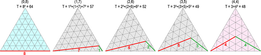
Geodesic polyhedra are defined by the equilateral triangles of the primary face (i.e., the face of the underlying tetrahedron, octahedron, or icosahedron) laid out on a 60° grid so that their vertices always align with grid crossings. This produces three classes of tiling or tessellation. The edges of the primary triangular face in Class 1 are parallel to the grid lines. The edges in Class 2 are perpendicular to the grid lines. Those in Class 3 are neither parallel nor perpendicular to the grid lines.
Geodesic polyhedra are divided into the three Classes defined by the orientation of the primary face laid out on a 60° grid. The edges of Class 1 polyhedra are parallel to the grid, Class 2 are perpendicular, and Class 3 skewed, neither parallel nor perpendicular to the grid.
The frequency of each class is given by two numbers (b,c) representing the number of triangular modules along the grid lines connecting adjacent vertices. The general formula for the area, or the number of triangular modules that subdivide the primary face, is given by:
Area (T) = b² + c² + (b×c)
For Class 1, b is the edge length of the primary face; so, c is always 0 and the formula reduces to b². For Class 2, b = c, so the formula can be reduced to 3b².
The frequency of each Class of geodesic polyhedron is given by two numbers (shown in parentheses) representing the number of triangular subdivisions along grid lines connecting adjacent vertices (red and green lines). The primary face of the F8 polyhedra in Class 1 (blue), Class 3 (gray), and Class 2 (pink) are shown, along with their areas (T).
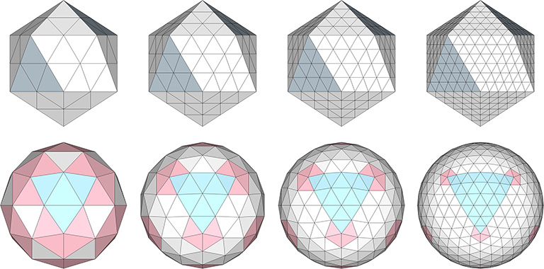
Class 1 Geodesics
Class 1 geodesics subdivide the primary face with lines parallel to the edges.
2F, 3F, 4F and 6F Class 1 geodesic polyhedra (icosahedron base)
Class 2 Geodesics
Class 2 geodesics subdivide the primary face with lines perpendicular to the edges.
2F, 4F, 6F, and 8F Class 2 geodesic polyhedra (icosahedron base)
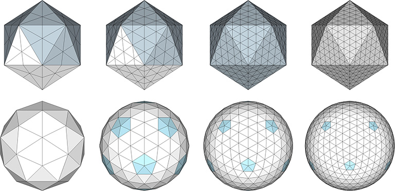
Class 3 Geodesics
Class 3 geodesics subdivide the face with lines that are askew to the edges, neither parallel no perpendicular.
3F, 4F, 6F, and 8F Class 3 geodesic polyhedra (icosahedron base)
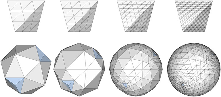
All of the geodesic polyhedra above have as their base the regular icosahedron. Being the most spherical, the icosahedron generates the most uniform tessellations. But the geodesic polyhedra may also be generated using the tetrahedron as their base, as in the following examples:
3F, 4F, 8F, and 16F Class 1 geodesic polyhedra (tetrahedron base)
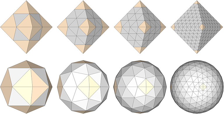
And they may also be generated using the octahedron as their base, as in these examples:
2F, 3F, 4F, and 8F Class 1 geodesic polyhedra (octahedron base)
The spherical tensegrities, whether based on the tetrahedron, octahedron, or icosahedron, have the shape of Goldberg polyhedra, the duals of geodesic polyhedra. Fuller held that all of his geodesic domes were, structurally, tensegrities. But then, any self-supporting structure can be described as a tensegrity. That is, all structural arrangements of vectors can be described as islands of compression in a continuous web of tension. Perhaps Fuller meant that his calculations were done on the spherical tensegrities, i.e., the tensor equilibrium phases of the tensegrity forms of the geodesic polyhedra. (See: Tensegrity, and; Tensegrity Equilibrium and Vector Equilibrium.) Many of Fuller’s domes do, in fact, have the appearance of Goldberg polyhedra. Fuller’s geodesic structures may be most accurately described as tensegrity composites incorporating both their spherical and polyhedron states.
The 2F Class 1 geodesic polyhedron as a Tensegrity composite, incorporating the 30-strut tensegrity sphere with its polyhedron counterpart, the tensegrity icosahedron.
An alternate construction of the 2F Class 1 geodesic polyhedron is achieved by reducing the the 120-strut tensegrity sphere to its polyhedron phase.
The 120-strut tensegrity sphere reduced to a 2F Class 1 geodesic polyhedron
Composite tensegrities, incorporating the spherical (Goldberg) and polyhedron (geodesic) phases of two or more frequencies may be possible without one interfering with the other. These may be easier to construct and would no doubt have incredible strength.