“Vector equilibrium accommodates all the inter-transformings of any one tetrahedron by polar pumping, or turning itself inside out. Each vector equilibrium has four directions in which it could turn inside out. It uses all four of them through the vector equilibrium’s common center and generates eight tetrahedra. The vector equilibrium is a tetrahedron exploding itself, turning itself inside out in four possible directions. So we get eight: inside and outside in four directions. The vector equilibrium is all eight of the potentials.”
—R. Buckminster Fuller, Synergetics, 441.02

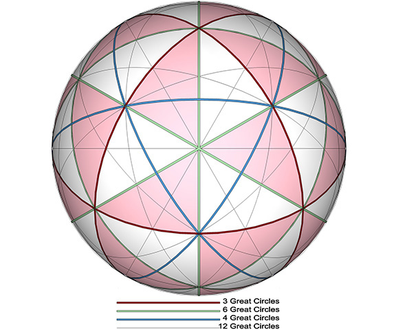
The axes of the set of 4 great circles of the vector equilibrium (VE) stands apart from the other three sets in its significance to the rest of Fuller’s geometry:

• It is the axis on which the vector model rotates and contracts in the jitterbug transformation. (See: Jitterbug.)
• Each of its four great circles passes through six of the twelve points of tangency between radially close-packed spheres, making it the most versatile of what Fuller called “railroad tracks of energy” in the isotropic vector matrix. (See: Great Circles: The 25 Great Circles of the Vector Equilibrium (VE); and The 25 Great Circles of the VE (new illustrations).)
• It is the only axis that connects nuclei directly to other nuclei, and forms the 14-around-1 rhombic dodecahedra matrix on which nuclei are distributed. (See: Formation and Distribution of Nuclei in Radial Close-Packing of Spheres.)
• It is the only axis along which no single great circle route can be directly traced. (See: Inter-Sphere Connections via the 25 Great Circles of the VE.)
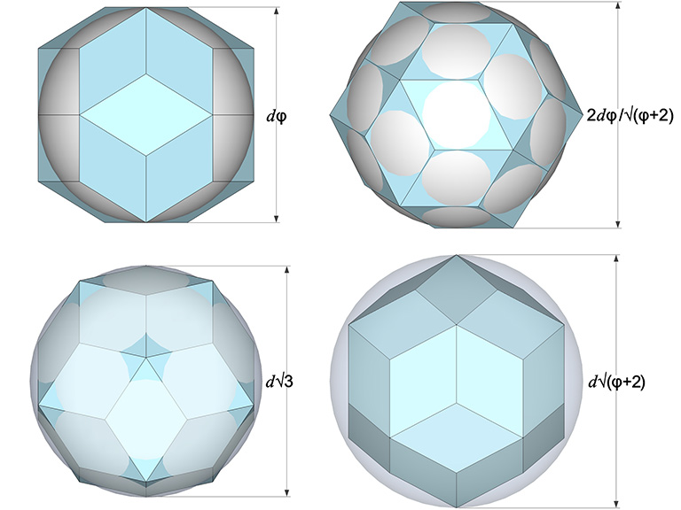
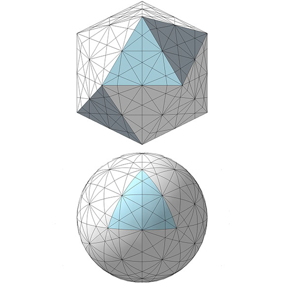
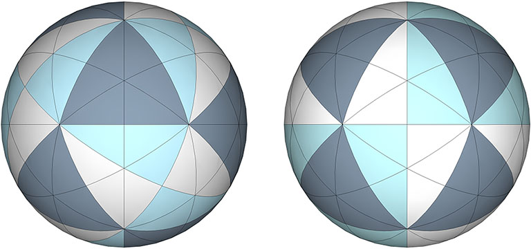
• Its four great circles define the spherical vector equilibrium.
• The combined area of its four great circle planes is identical with the surface area of the sphere of the same radius.
• The axis forms a channel for the polar pump model of the jitterbug transformation, which is the topic of this article.

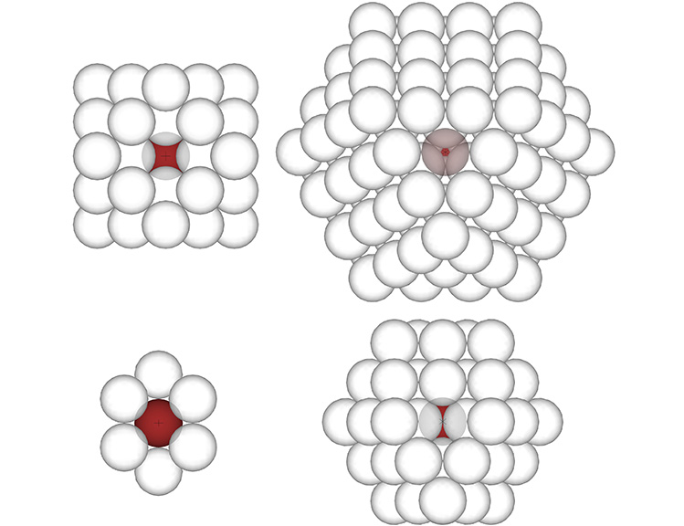
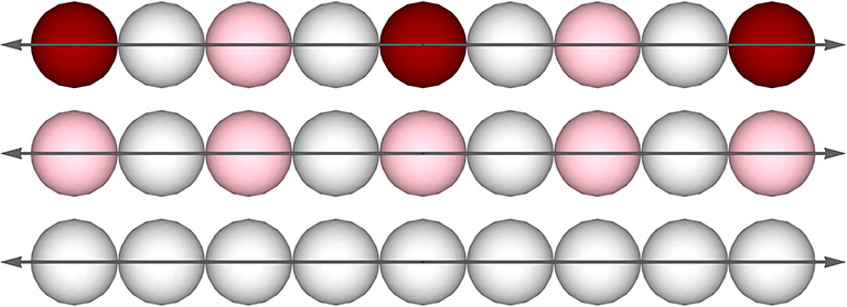
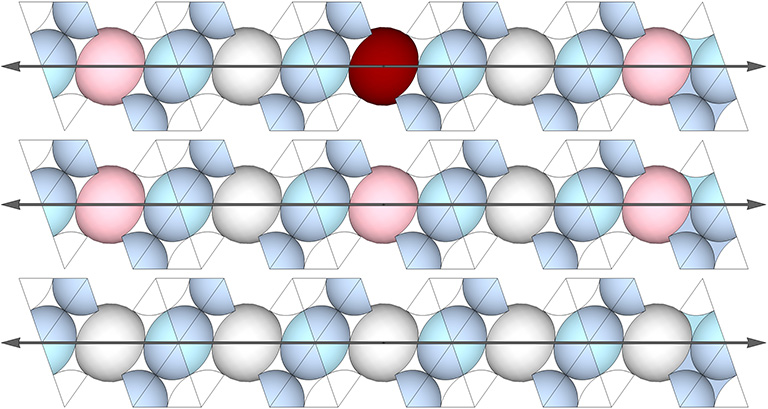
The primary axis of the set of four great circles directly connects each nucleus with 8 of its 14 surrounding nuclei with no intervening spheres between them. Its secondary axes also connect like spheres: nuclear voids with nuclear voids, and; F1 shell spheres with F1 shell spheres. (See: Categories of Spheres in the Isotropic Vector Matrix: Nuclei, F1 Shells, and “Nuclear Voids”). Each sphere is separated along each axis by interstitial space consisting of one concave VE and two concave octahedra. (See: Spaces and Spheres (Redux) and Spheres and Spaces.)

If we imagine the matrix shuttling spheres exclusively along these axes, each cycle of the jitterbug produces identical results and no change is perceived in the configuration or orientation of the discrete cubes and VEs described in my previous article, Blinkers, the Jitterbug, and the “Crystalized” Isotropic Vector Matrix.

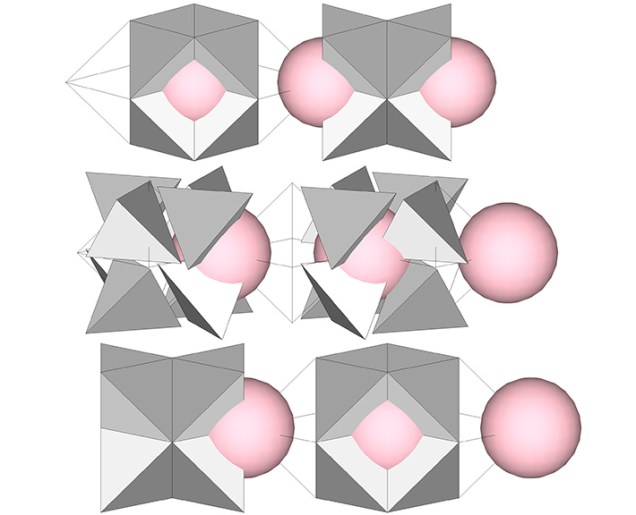
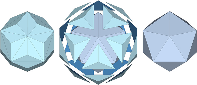
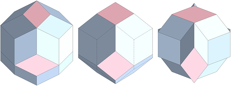
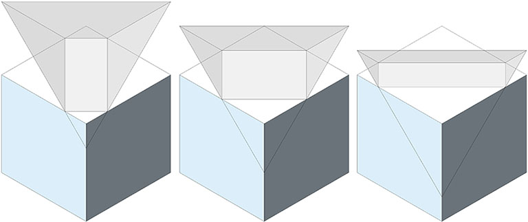
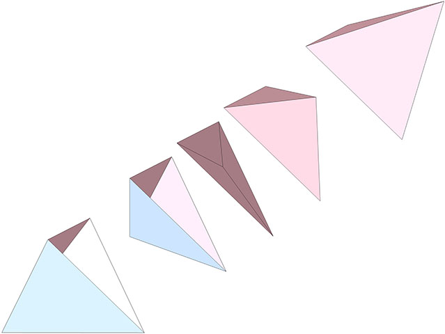
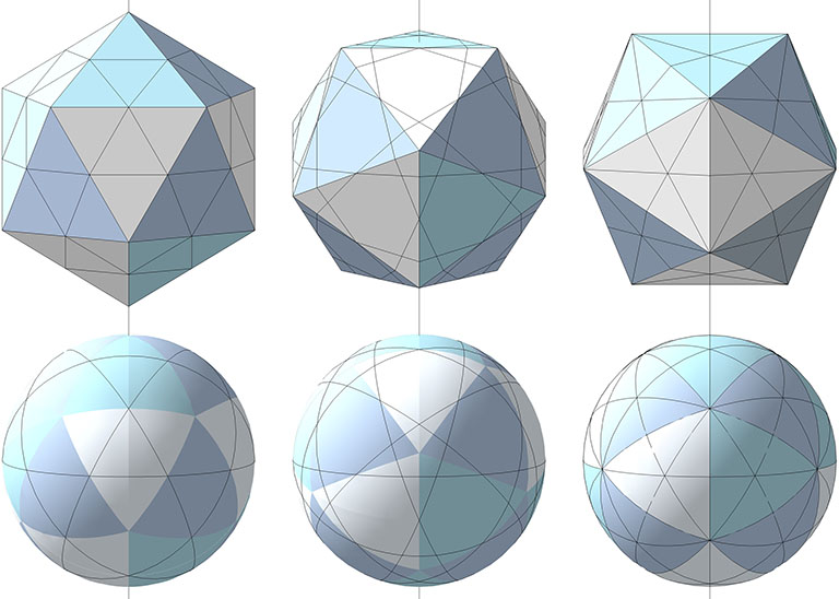
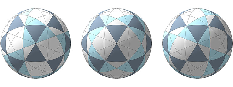
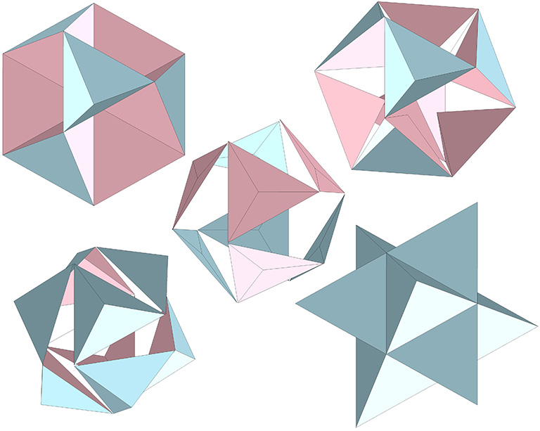
The jitterbug is, essentially, the positive-negative oscillation of tetrahedra, and Fuller consistently viewed this oscillation as the vector equilibrium (VE) exploding itself, its eight tetrahedra forcing their common vertex out through their opposite faces to form the star octahedron, or cube, as illustrated below.

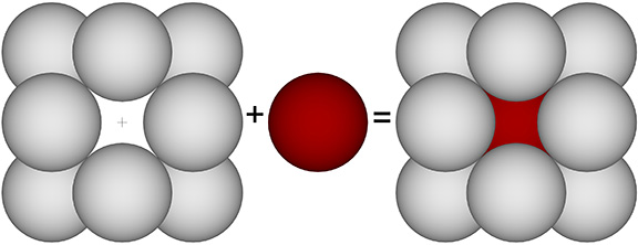
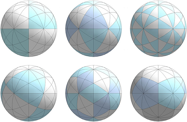
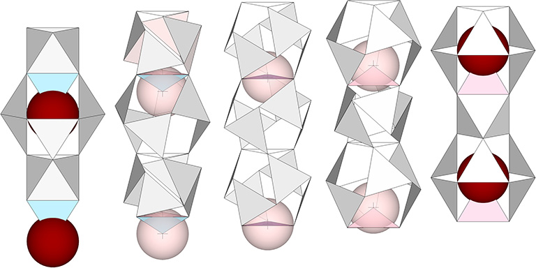
The following illustrates how this model of the jitterbug might be conceived as the shuttling of nuclei into and out of the octahedra as they unfold into VEs and fold back again into octahedra. This is the same space-to-sphere, sphere-to-space oscillation as in all other models of the jitterbug—the only difference being the axis along which the adjacent space (the concave VE that is replaced by a sphere) is perceived to lie.

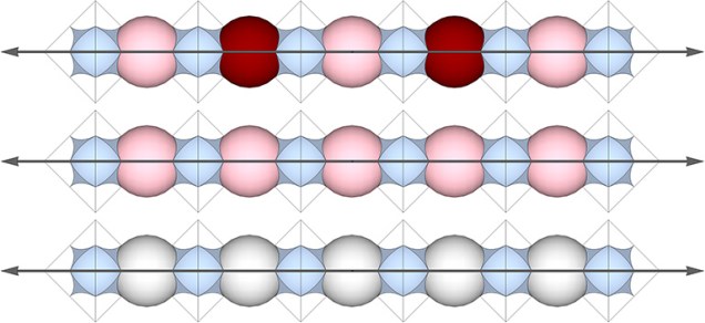
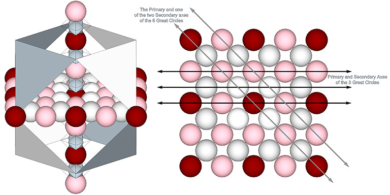
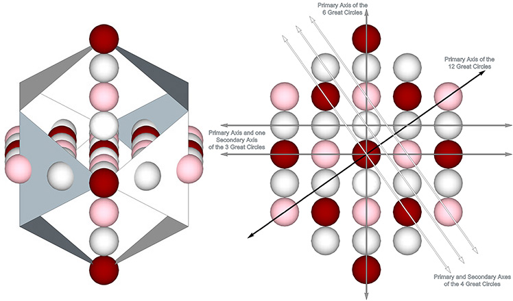
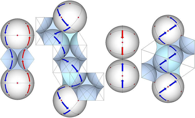
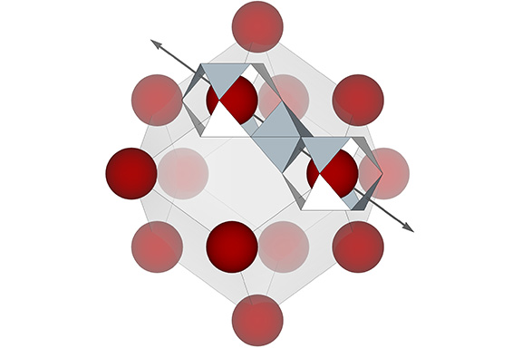
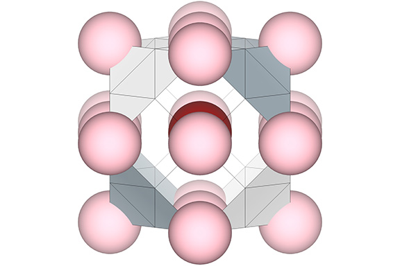
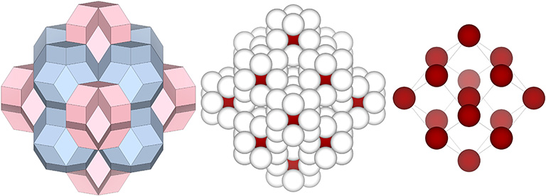
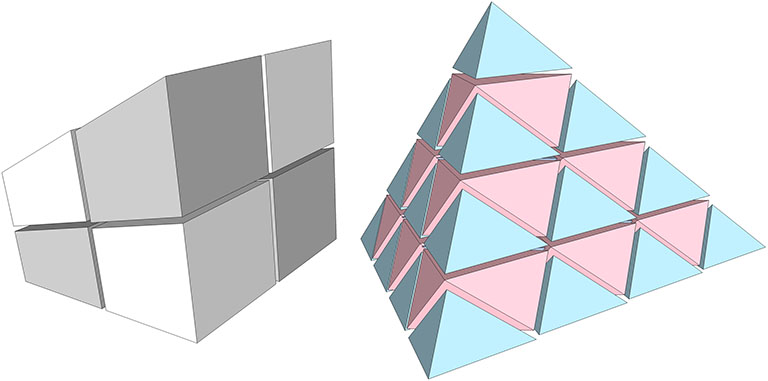
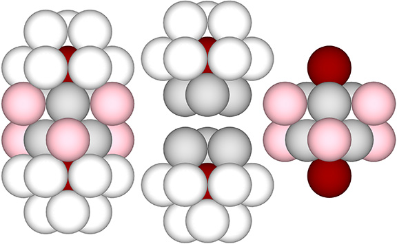
In the illustration below, the six spheres of the octahedron (gray spheres) contribute 3-spheres each to the F1 shells of two nuclei (center) aligned on opposing points of each of the cube’s (right) four diagonals, one of which is the primary axis of the four great circles connecting nuclei (red spheres), and the others are secondary axes connecting nuclear voids (pink spheres). This polarization of the nuclei to just one of the four axes may explain why Fuller referred to its migration along this axis as a “polar” pump.

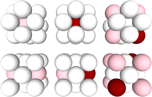
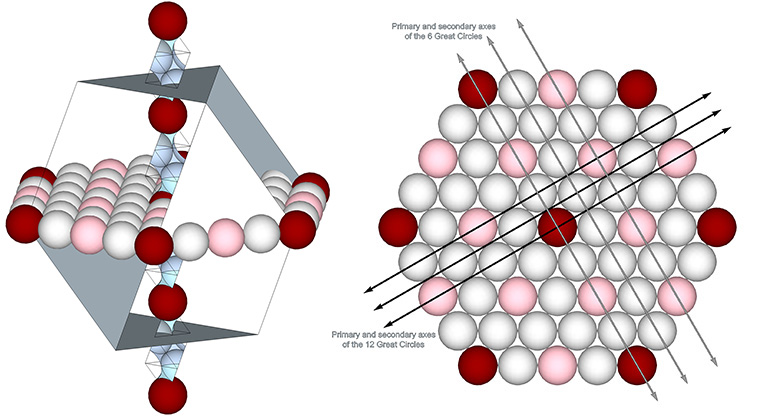
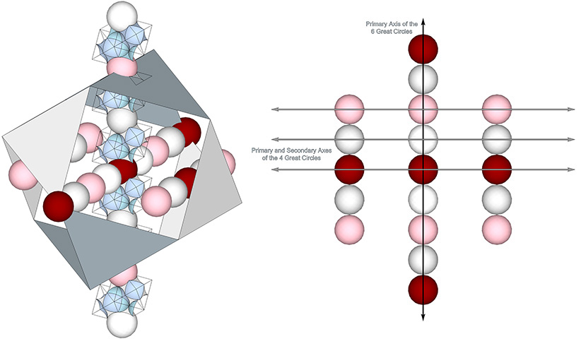
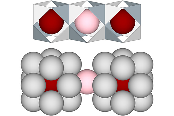
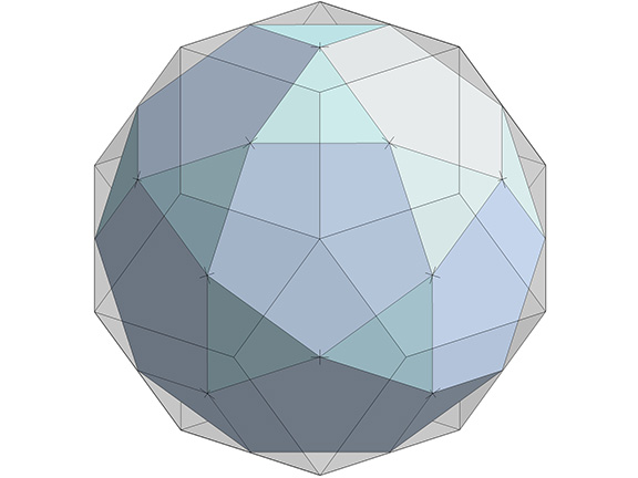
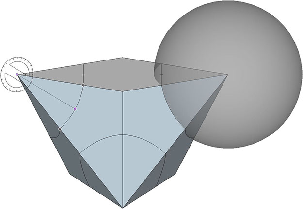
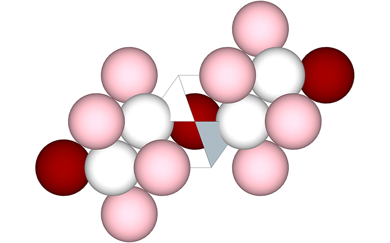
In the following illustration, two of these polarized cubes are shown straddling a VE with which they share a nucleus.

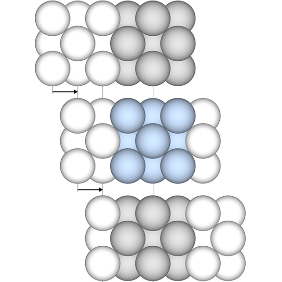
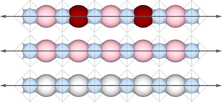
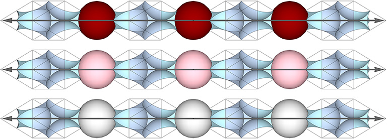
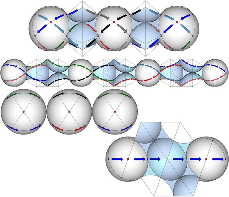
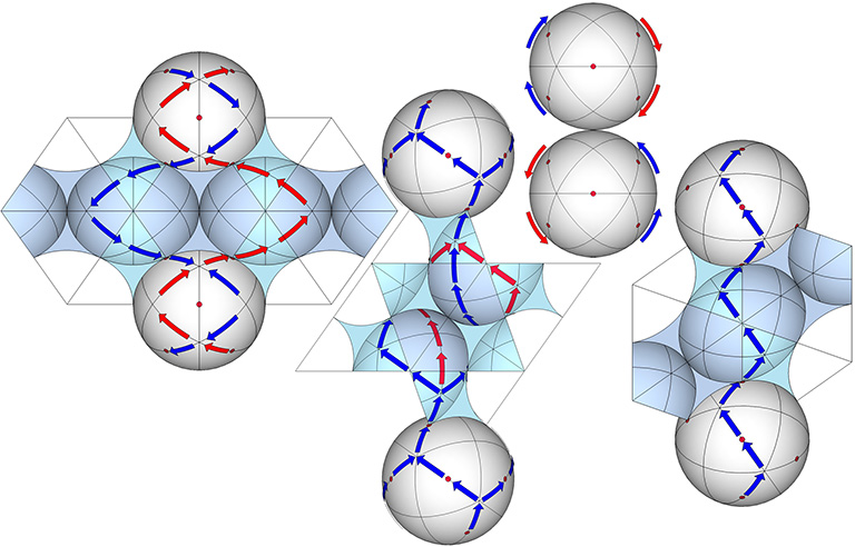
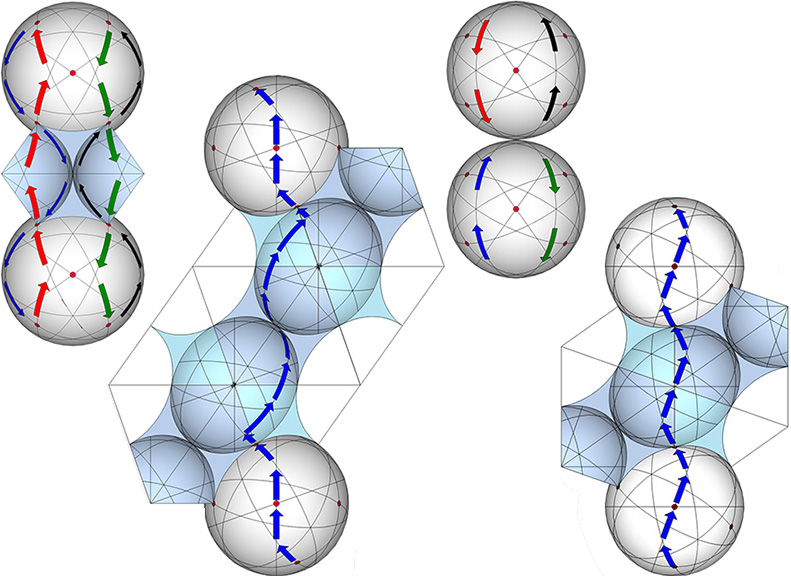
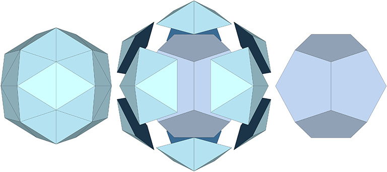
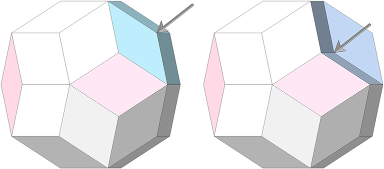
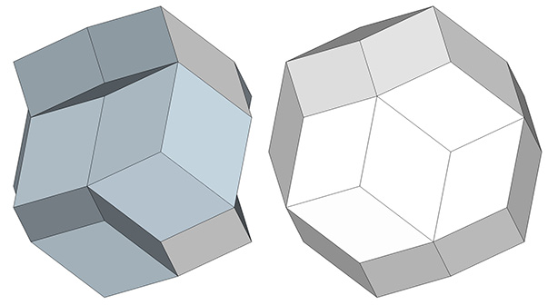
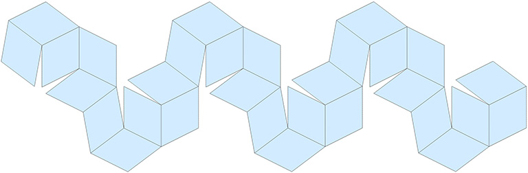
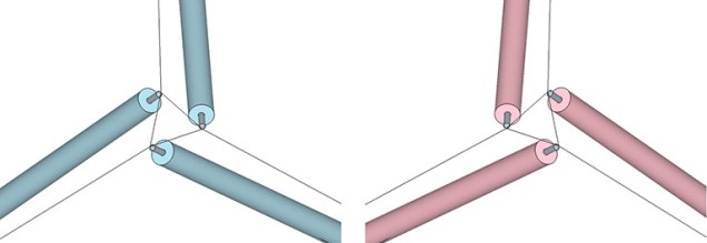
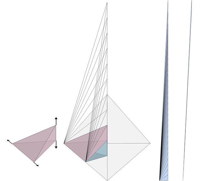
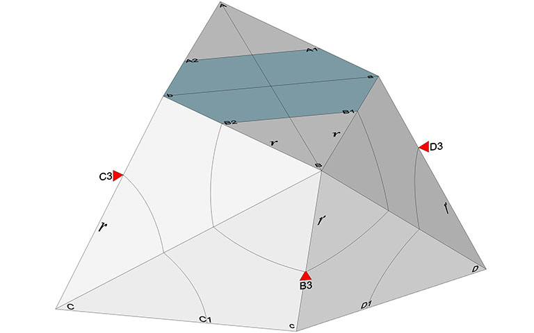
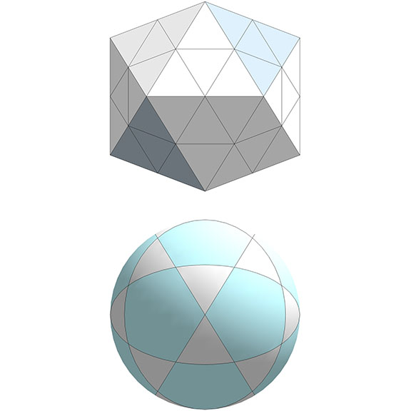
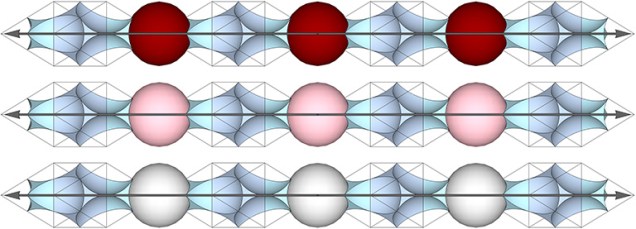
At the top of the illustration below, the cubic clusters of close-packed spheres have been replaced with octahedra, inside of which are the inside-outed tetrahedra from their adjacent VEs. Below that, the octahedra and tetrahedra have been replaced with concave VE spaces and concave octahedron interstices. Arrows indicate how the set of four great circles constitute the shortest-distance geodesics connecting spheres along the axis. Note that the path makes a sharp right angle at the halfway point. For each of the eight possible geodesics (for which only one is shown), the red arrows change to blue arrows at the point of tangency between two of the six spheres of the octahedron that sits between the VEs. This mirrors the positive-negative oscillations of tetrahedra.

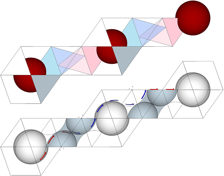
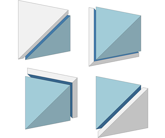
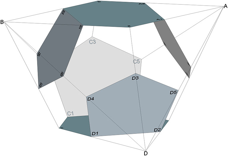
Another way of looking that this is to have the tetrahedra unfold and wrap themselves around the octahedra, then unwrap and refold themselves into tetrahedra at the octahedron’s opposite pole.

The octahedron sits between a positive and a negative tetrahedron in the isotropic vector matrix, and accommodates their inside-outing, or positive-negative oscillations, both internally, i.e., as inside-outed tetrahedra clustered inside the octahedron, and externally, i.e., as tetrahedra unfolded and wrapped around its surface. The model provides a way of visualizing the jitterbug transformation on an otherwise fixed matrix.

“We may define the individual as one way the game of Universe could have eventuated to date. Universe is the omnidirectional, omnifrequency game of chess in which with each turn of the play there are 12 vectorial degrees of freedom: six positive and six negative moves to be made. This is a phenomenon of frequencies and periodicities. Each individual is a complete game of Universe from beginning to end.”
—R. Buckminster Fuller, Synergetics, 537.41

In previous posts, I’ve suggested that the jitterbug transformation may be associated with the migration of nuclei. The radially close-packed spheres of the isotropic vector matrix divide naturally into clusters in the shape of cubes and vector equilibria (VEs). See Space-Filling Polyhedra as Close-Packed Spheres. In the following illustration I’ve replaced the sphere clusters with tetrahedra. The eight tetrahedra that share a common vertex at the center of the VE are rotated 90°, or “jitterbug”, so that their common vertex faces outward to form the eight points of the cube. If we add the nuclei into this model, it suggests a migration of nuclei between the two.

The effect of the jitterbug transformation may also be conceived as the shifting not only of nuclei but of all spheres comprising the isotropic vector matrix into their adjacent spaces. The natural axis for the transformation is that of the 3 Great Circles, the only axis on which every sphere is connected directly through the center of a space, i.e., a concave VE. (See: Spheres and Spaces, and Spaces and Spheres (Redux).)

To see the outcome of the transformation, we need only shift our perspective—or hold our perspective constant while the matrix makes a lateral shift—left, right, up, down, in, or out—the distance of √2×r, where r is the radius of the sphere. In the illustration below we see a cube (blue) occupying the space previously occupied by a VE (gray), and then a VE (gray) again.

The identification of any single nucleus will have the effect of defining every other sphere in the isotropic vector matrix (see Formation and Distribution of Nuclei in Radial Close-Packing of Spheres). Nuclei are defined by their 12-sphere shells, and the remaining spheres (those that are neither a nucleus nor a sphere in a nucleus’s shell) are categorized as nuclear voids, i.e., nuclei whose shells consist entirely of spheres from the shells of their surrounding nuclei. (See Categories of Spheres in the Isotropic Vector Matrix: Nuclei, F1 Shells, and “Nuclear Voids”.) Implicit in the identification of any given sphere as a nucleus is the categorization of every other sphere; identifying a nucleus effectively “crystalizes” the matrix. Crystal lattices and networks are famously dull; the part tells the story of the whole. It is the jitterbug that makes it interesting.

As I said above, radially close-packed spheres divide naturally into vector equilibria and cubes, and we may think of one becoming the other in the jitterbug. In a “crystalized” matrix, we find three variations of each, i.e, three unique VEs and three unique cubes, each with a unique arrangement of the three categories of sphere. These I’m calling “blinkers,” borrowing from the lexicon of the legendary Game of Life which was developed by mathematician John Horton Conway in 1970.

As the matrix jitterbugs, one cube or VE will be replaced with another—different, or the same rotated from its original orientation. They will appear to blink, flash, rotate, and oscillate as spheres are replaced by spaces and the spaces are replaced, again, by spheres. The jitterbug, in effect, can generate an infinite number of patterns that are replicated and regenerated throughout the matrix. In effect, the dull crystal is made into a kind of neural network by this interpretation of the jitterbug transformation.

“The first layer consists of 12 spheres tangentially surrounding a nuclear sphere; the second omnisurrounding tangential layer consists of 42 spheres; the third 92, and the order of successively enclosing layers will be 162 spheres, 252 spheres, and so forth. Each layer has an excess of two diametrically positioned spheres which describe the successive poles of the 25 alternative neutral axes of spin of the nuclear group.”
— R. Buckminster Fuller, Synergetics, 222.23

The four sets of 3, 4, 6, and 12 axes that define the 25 great circles of the vector equilibrium also comprise all line-of-sight connections between spheres radially close-packed in the isotropic vector matrix. That is, each axis proceeds directly, without deviation, through interstitial space from one sphere center to the next. This may be made more clear with the following illustration.

In the above illustration,

• The axis for the 3 great circles (top left) connects the semi-transparent sphere in the F2 layer with the nucleus (red), having passed through interstitial space in the F1 layer. Note that this is the only axis that provides a direct connection between nuclei and nuclear voids (see Categories of Spheres in the Isotropic Vector Matrix: Nuclei, F1 Shells, and “Nuclear Voids”). The semi-transparent sphere in the F2 layer will be surrounded by the F1 shells of its surrounding nuclei, and therefore qualifies as a nuclear void.
• The axis of the 4 great circles (top right) connects the semi-transparent sphere in the F3 layer with the nucleus (red) after having passed through interstitial space in both the F2 and F1 layers. Note that this is the only axis that provides a direct connection between nuclei; the semi-transparent sphere in the F3 layer will have its own layer of 12 spheres, and therefore qualifies as a nucleus.
• The axis of the 6 great circles (bottom left) is unique in that it forms an unbroken chain of spheres in direct contact with one another. The semi-transparent sphere in the F1 shell is in direct contact with the nucleus.
• The axis of the 12 great circles (bottom right) connects the semi-transparent sphere in the F2 layer with the nucleus after having passed through what Fuller calls the “kissing point”, i.e., the point of contact between two spheres in the F1 layer.

Set of 3 Great Circles of the VE

The axes of the 3 great circles pass through the centers of opposing square faces of the VE. Its primary axis connects nuclei in every fourth layer. Their great circle planes are in alignment with the three unique axes for the 3 Great Circles, and two of the three unique axes for the 6 Great Circles.

The axes pass alternately through a space (concave VE) and a sphere (convex VE). On the primary axes, the spheres alternate between nuclei (shown in red) and nuclear voids (pink). On the two secondary axes (those that do not pass through a nuclear sphere), the spheres are either all nuclear voids (pink) or spheres that occupy the F1 shells of nuclei. Shell spheres are shown in white. (See: Categories of Spheres in the Isotropic Vector Matrix: Nuclei, F1 Shells, and “Nuclear Voids”.)

Set of 4 Great Circles of the VE

The axes of the 4 great circles pass through the centers of opposing triangular faces of the VE. Its primary axis connects nuclei in every 3rd layer. Their great circle planes are in alignment with the three unique axes for the sets 6 and 12 Great Circles.

The primary axis joins nuclei. The secondary axes join nuclear voids or shell spheres. Between each sphere on the axes is interstitial space consisting of a space (concave VE) flanked by one positive and one negative interstice (concave octahedra). See: Spheres and Spaces, and; Spaces and Spheres (Redux).

The axis of the set of four great circles is unique in that no single geodesic path directly joins the spheres along the axis. See Inter-Sphere Connections via the 25 Great Circles of the VE.

Set of 6 Great Circles of the VE

The axes of the 6 Great Circles pass through opposing vertices of the VE. Its primary axis connects nuclei in every fourth layer. Their great circle planes are in alignment with the three unique axes of the 4 Great Circles, the primary axis and and one secondary axis of the 3 great circles, and the primary axis of the 6 and 12 Great Circles.

The primary axis joins nuclei and nuclear voids between each of which is a shell sphere. One secondary axes joins nuclear voids each separated by a shell sphere, and the other secondary axis forms an unbroken chain of shell spheres.

Set of 12 Great Circles of the VE

The axes of the 12 Great Circles pass through the centers of opposing edges of the VE. Its primary axis connects nuclei in every fifth layer. Their great-circle planes are in alignment with the three unique axes of the 4 Great Circles, and the primary axis of the 6 Great Circles.

Primary and secondary axes of the 12 great circles follow the same pattern as the axes of the 6 great circles, but with all all spheres separated by interstitial space.

Knowing how the three categories of spheres are distributed along the primary axes should enable us to count the total number of nuclei in each shell of the vector equilibrium. The primary axes for the sets of 3 and 6 Great Circles pass through a nucleus with every fourth shell. The primary axis for the Set of 4 Great Circles passes through a nucleus with every third shell And, the primary axes of the set of 12 Great Circles pass through a nucleus with every eighth shell. It follows that only those shells which are multiples of 3, 4 and 8 contain nuclei. The F1, F2, and F5 shells, for example, have none. We also know that nuclei are evenly distributed on a grid of rhombic dodecahedra (see Formation and Distribution of Nuclei in Radial Close-Packing of Spheres), and that the shell growth formula for the rhombic dodecahedron is 12F²+2 (see Concentric Sphere Shell Growth Rates). If anyone knows, or is able to derive the formula, please share.

“Whereas each of the 25 great circles of the vector equilibrium go through the 12 vertexes at least twice; and whereas the 12 vertexes are the only points of inter-tangency of symmetric, unit-radius spheres, one with the other, in closest packing of spheres; and inasmuch as we find that energy charges always follow the convex surfaces of systems; and inasmuch as the great circles represent the most economical, the shortest distance between points on spheres; and inasmuch as we find that energy always takes the most economical route; therefore, it is perfectly clear that energy charges passing through an aggregate of closest-packed spheres, from one to another, could and would employ only the 25 great circles as the great circle railroad tracks between the points of tangency of the spheres, ergo, between points in Universe. We can say, then, that the 25 great circles of the vector equilibrium represent all the possible railroad tracks of shortest energy travel through closest-packed spheres or atoms.”
—R. Buckminster Fuller, Synergetics, 458.01

Fuller proposed that the 25 great circles of the vector equilibrium account for all the routes by which energy is transmitted between spheres in the isotropic vector matrix. Or, to put it more dramatically, the great circles defined by the four sets of 3, 4, 6 and 12 spin axes of the VE represent all possible tracks of shortest energy travel between points in the universe.

See: Great Circles: The 25 Great Circles of the Vector Equilibrium (VE), and; The 25 Great Circles of the VE (new illustrations)

All great circle trajectories may be reduced to combinations of the shortest-distance paths for each set of great circles connecting adjacent spheres on each of the four axes. (See Distribution of Radially Close-Packed Spheres on the 25 Axes and Great Circle Planes of the Vector Equilibrium.)

The Set of 3 Great Circles

The great circles in the set of 3 are defined by spin axes running through the centers of opposing square faces of the VE. Each great circle passes through four vertices and therefore has four opportunities with each 360° circuit to connect to an adjacent sphere.

• On the axis of the 3 great circles, the set of 3 reveals four equally efficient paths, two of which are shown below (left).
• On the axis of the 4 great circles, the set of 3 reveals six equally efficient paths, one of which is shown in below (left middle).
• All of the great circle sets connect spheres on the axis of the 6 great circles with equal efficiency, differing only in the number of alternate paths; the set of 3 (right middle), reveals two.
• On the axis of the 12 great circles, the set of 3 reveals two equally efficient paths, one of which is shown below (right).

The Set of 4 Great Circles

The great circles in the set of 4 are defined by spin axes running through opposing triangular faces of the vector equilibrium (VE). Each great circle passes through six vertices and therefore has six opportunities with each 360° circuit to connect with an adjacent sphere.

• On the axis of the 3 great circles (top), the set of 4 reveals eight equally-efficient helical routes that complete a cycle every other sphere.
• On the axis of the 4 great circles (middle top), the set of 4 reveals eight equally-efficient helical routes the complete a cycle every fourth sphere.
• On the axis of the 6 great circles (middle bottom), the set of 4 reveals four equally-efficient routes between spheres.
• On the axis of the 12 great circles (bottom), the set of 4 reveals two equally-efficient routes between spheres.

The Set of 6 Great Circles

The great circles in the set of 6 are defined by spin axes running through opposing vertices of the vector equilibrium (VE). Each great circle passes through two diametrically opposed vertices.

• On the axis of the 3 great circles, the set of 6 (left) reveals 4 equally-efficient routes between spheres.
• On the axis of the 4 great circles, the set of of 6 (middle left) reveals a branching network of at least 36 equally-efficient paths.
• On the axis of the set of 6 great circles, the set of 6 (middle right) reveals two equally-efficient paths between spheres.
• On the axis of the 12 great circles, the set of 6 (right) reveals two equally-efficient paths between spheres.

The Set of 12 Great Circles

The great circles in the set of 12 are defined by spin axes running through the midpoints of opposing edges of the vector equilibrium (VE). As with the set of 6, each great circle in the set of 3 passes through two diametrically opposed vertices.

• On the axis of the set of 3 great circles (left), the set of 12 reveals eight equally-efficient routes between spheres.
• On the axis of the 4 great circles (middle left), the set of 12 reveals four equally-efficient paths, one of which is shown.
• On the axis of the set of 6 great circles (middle right), the set of 12 reveals four equally-efficient paths.
• On the axis of the set of 12 great great circles (right), the set of 12 reveals two equally-efficient paths, one of which is shown.

When modeling the distribution of nuclei in the isostropic vector matrix, I distinguish between the nuclei and the 12-sphere shells that isolate and define them. These nuclear domains, each consisting of one nuclear sphere and a 12-sphere shell, defines the vector equilibrium, or VE.

Nuclei are distributed throughout the isotropic vector matrix at the centers and vertices of close-packed rhombic dodecahedra whose edges align with the primary axes of of the vector equilibrium’s 4 great circles. See: Formation and Distribution of Nuclei in Radial Close-Packing of Spheres; and Great Circles: The 25 Great Circles of the Vector Equilibrium (VE); The 25 Great Circles of the VE (new illustrations); and Distribution of Radially Close-Packed Spheres on the 25 Axes and Great Circle Planes of the Vector Equilibrium.

Nuclei and their shells do not close-pack to fill all-space. Between these nuclear clusters are gaps which combine for form holes that run laterally through the isotropic vector matrix.

The spheres that fill these voids can be isolated to show that they all lie on a cubic grid which follows the square-face diagonals of close-packed F2 VEs.

I refer to these as “nuclear voids” because, like the nuclei, each occupies the center of a VE, but unlike the nuclei, they do not have their own 12-sphere shells. Rather, every sphere in direct contact with a “nuclear void” is uniquely identified with the shell of one of its neighboring nuclei.

The rhombic triacontahedron has 30 faces, 60 edges, and 32 vertices. Each of its 30 faces is a golden rhombus, i.e., the length of its long diagonal is related to the length of its short diagonal by φ, the golden ratio: (√5+1)/2 ≈ 1.61803398875

If the long diagonal is taken as d, the length of its short diagonal is d/φ. Its face angles are atan(2) ≈ 63.434948823°, and 2atan(φ) ≈ 116.565051177°. Its dihedral angle is 144°.

The central angle of its long diagonal, d, is atan(2) ≈ 63.434948823°. The central angle of its short diagonal, d/φ, is atan(2/√5) ≈ 41.810314896°. The central angle of its edge, a, is atan(2/φ²) ≈ 37.377368141°.

The in-sphere diameter is dφ. The mid-sphere diameter is 2dφ/√(φ+2). The circum-sphere diameter, i.e., the diameter measured by connecting opposite vertices bounded by four rhomboid faces, is d√(φ+2). The diameter measured by connecting opposite vertices bounded by three rhomboid faces, is d√3.

φ = Golden Ratio = (√5+1)/2

Dimensions in units of edge length, a:

• a = edge length
• Volume (cubic) = a³ × 4√(5+2√5)
• Volume (tetrahedral) = a³ × 4√(5+2√5) × 6√2
• In-sphere radius = a × φ²/√(1+φ²) = φ/√(3-φ)
• Circumsphere radius r = a × φ
• Circumsphere radius r‘ = a × φ√(3/(φ+2))
• Mid-sphere radius = a × 2φ/√5

Dimensions in units of the long diagonal, d:

• d = long diagonal
• Volume (cubic) = d³ × 5/2
• Volume (tetrahedral) = d³ × 15√2
• In-sphere radius = d × φ/2
• Circumsphere radius r = d × √(φ+2)/2
• Circumsphere radius r’ = d × √3/2
• Mid-sphere radius = d × 1/√(φ+2)

Identities:

• a = d × √(3-φ)/2
• d = a × 2/√(3-φ)
• d/φ = short diagonal

Truncating the rhombic triacontahedron on the long diagonal of its rhomboid face describes the regular icosahedron.

Truncating the rhombic triacontahedron on the short diagonal of its rhomboid face describes the pentagonal dodecahedron.

Connecting the face centers describes the icosidodecahedron.

When a concentrated load is applied radially (toward the center) to any vertex of a polyhedral system, it tends to cause a dimpling effect. As the frequency or complexity of the system increases, the dimpling becomes progressively more localized, and proportionately less force is required to bring it about.

The rhombic triacontahedron may be a limit case in which the dimpling of its eight three-vector vertices produces a concave rhombic triacontahedron that close-packs with the convex triacontahedron to fill all-space.

The convex and concave rhombic triacontahedra close-pack radially around a common center as rhombic dodecahedra, a pattern which is identical to the distribution of unique nuclei in the isotropic vector matrix. (See Formation and Distribution of Nuclei in Radial Close-Packing of Spheres.)

If the edge length is preserved, i.e., if we imagine the rhombic triacontahedron constructed of rigid struts and flexible connectors, it will undergo a jitterbug-like transformation into the all-space-filling Kelvin truncated octahedron at the halfway point in the transition between its convex and concave forms.

The in-sphere diameter of the rhombic triacontahedron with a tetrahedral volume of 5 is approximately 0.000517 less than the prime unit vector. This is an exquisitely small difference, and Fuller initially believed it to be due to the low resolution of the trigonometry tables he was using. The rhombic triacontahedron can be divided into 120 identical tetrahedra, and with a tetrahedral volume of five, each of the these 120 tetrahedra would have precisely the same volume as the A and B quanta modules, i.e., 1/24th of a unit tetrahedron. These he called the T quanta modules (‘T’ for ‘Triacontahedon’).

Subsequent calculations proved that the rhombic triacontahedron with a unit in-sphere diameter would have a tetrahedral volume of slightly more than 5. So, though his T quanta modules had a rational volume of 1/24th of the unit tetrahedron, the dimension corresponding to the in-sphere radius was awkward and irrational. The quanta module derived from the rhombic dodecahedron with a unit in-sphere diameter was subsequently named the E quanta module (‘E’ for ‘Einstein’). See T and E Quanta Modules.

For a rhombic triacontahedron with a tetrahedral volume of 5:

• 120 T quanta modules
• d = ³√(√2/6)
• In-sphere diameter = dφ ≈ 0.999483332262

For a rhombic triacontahedron with an in-sphere diameter of 1:

• 120 E quanta modules
• d = φ-1
• Volume (tetrahedral) = d³ ×15√2 = (φ-1)³ × 15√2 ≈ 5.007758031333.

The rhombic triacontahedron may be unspooled into a continuous chain of rhombuses.

The construction is accomplished by 29 sequential folds of 36°.

The tetrakaidecahedron of the Weaire-Phelan structure complements the pyritohedron to fill all-space. Together, they constitute what is presently determined to be the best solution to the Kelvin Problem: How can space be partitioned into cells of equal volume with the least area of surface between them?

In previous articles, I demonstrated that the pyritohedra of the Weaire-Phelan structure align perfectly with the distribution of unique nuclei in the radial close-packing of spheres of the isotropic vector matrix. See: Formation and Distribution of Nuclei in Radial Close-Packing of Spheres; Tetrakaidecahedron and Pyritohedron; and Kelvin Truncated Octahedron. I was able to relate the two matrices and rationalize their volumes with reference to the variable, d, the diameter of the unit spheres of the isotropic vector matrix, and the constant α = ³√(√2/2), the length of the pyritohedron’s long edge when d is taken as unity. See: Pyritohedron Dimensions and Whole-Number Volume.

To summarize my conclusions:

• If the sphere diameter, d, is taken as unity, the tetrahedral volumes of both the pyritohedron and the tetrakaidecahedron of the Weaire-Phelan structure work out to be precisely 24d³.

• If its longest edge, a, is taken as unity, then d = 1/α, and the cubic volumes of both the pyritohedron and the tetrakaidecahedron of the Weaire-Phelan structure work out to be precisely 4a³.

To satisfy the Kelvin problem, the volumes of the two shapes, i.e., the pyritohedron and its complementary tetrakaidecahedron, must be identical. This tetrakaidecahedron has three unique faces: two hexagonal faces; four large pentagonal faces; and eight smaller pentagonal faces, for a total of 14 faces — tetra (four), kai (+), deca (ten), hedron (face). To determine its volume, we’ll need the areas and in-sphere radii for each of its faces.

• in-sphere radius to hexagonal face: d × √2/2
• in-sphere radius to larger pentagonal face: d × ≈ 0.784294792 *
• in-sphere radius to smaller pentagonal face: d × √3/2

* Though it should be possible to work out its precise value algebraically, I have so far been unsuccessful in resolving the in-sphere radius for the larger of the two pentagonal faces into whole number radicals and ratios.

In addition to the in-sphere radii as shown above, we must calculate the surface area for each of the faces. This is most easily accomplished by dividing each face into right triangles.

The hexagonal face is divided into four right triangles and one rectangle as follows:

• Four right triangles of atan(1/2), with legs measuring d(√2/α) and d(√2/α)/2.
• One rectangle measuring 2d(√2/α) by (d × α).

The larger of the two pentagonal faces is divided into four right triangles and one rectangle as follows:

• Two right triangles of atan(√5/4) with legs measuring d(α√5/6) and d(2α/3).
• Two right triangles of atan(√5/10) with legs measuring d(α/6) and d(α√5/3).
• One rectangle measuring d(α√5/3) by (d × α).

The smaller of the two pentagonal faces is divided into four right triangles and one rectangle as follows:

• Two right triangles of atan(√6/3) with legs measuring d(α√5/6) and d(2α/3).
• Two right triangles of atan(√6/6) with legs measuring d(α/√2) and d(α√3/6).
• One rectangle measuring d√3(√2-4α/3) by d(α/√2).

If d is taken as unity (d = 1), then a = d × α = ³√(√2/2), and

• The hexagonal face has a square area of ≈ 1.20629947402.
• The cubic volume of its polyhedral cone is area/3 × √2/2 ≈ 0.28432751274
• Multiplying by 2 (for the two hexagonal faces) ≈ 0.56865502548
• Converting from cubic to tetrahedral units, multiply the above volume by 6√2 ≈ 4.825197896
• Applying the same calculations to the large pentagonal faces, gives a total tetrahedral volume of 7.874010518.
• And, applied to the small pentagonal faces, gives a total tetrahedral volume of 11.30079158.
• 4.825197896 + 7.874010518 + 11.30079158 = 24, and it therefore follows that its tetrahedral volume is 24d³.

If the long edge (the base of the larger pentagonal face) is taken as unity, the d in our equations = 1/α, then a = α/α = 1. The cubic volumes then are, respectively, 0.804199649, 1.312335086, and 1.883465264, and

• 0.804199649 + 1.312335086 + 1.883465264 = 4, and it therefore follows that its cubic volume is 4a³.

While irregular cubes subdivide into dissimilar six-sided polyhedra, any tetrahedron, regular or irregular, will always subdivide into similar tetrahedra and octahedra.

The perimeter of any rectangle defined by the section plane of a regular tetrahedron cutting perpendicularly through its edge-to-edge axis is a constant equal to 2 times its edge length.

Any tetrahedron, regular or irregular, may be sliced parallel to any one or more of its faces without losing its basic symmetry. Or, as Fuller observed, “only the tetrahedron’s four-dimensional coordination can accommodate asymmetric aberrations without in any way disrupting the symmetrical integrity of the system.” (Synergetics, 100.304)

The pulling outward or pushing inward of one or more faces of the tetrahedron accomplishes the same transformation as uniform scaling would achieve. This accommodation of asymmetrical aberrations while preserving its symmetrical integrity allows for the linear translation of the its center of gravity without actually moving the tetrahedron.

The illustration below shows the same transformation, but with the two actions performed simultaneously, i.e., the pulling outward of one face occurs at the same time and at the same rate as the other face is pushed inward. This is essentially equivalent to a linear translation of the tetrahedron. We can accomplish any translation to any coordinates using this method, something that is possible with no other polyhedron.

The tetrahedron may be turned inside out by pushing a vertex through the opening of its opposite face.

Each consecutive (non-oscillating) inside-outing produces a unique orientation of the tetrahedron, and results in an infinite or near-infinite number of helices or helical translations. See also: Tetrahelix.

The tetrahedron may also turn itself inside-out by rotating three of its triangular faces outward from their common vertex like the petals of a flower. The process may be halted before the vertices rejoin on the opposite side, with the result being an octahedron rather than another tetrahedron. In the octet truss network, the octahedra occupy the spaces between tetrahedra. In the isostropic vector matrix, the octahedron defines the space between the spheres which in turn are defined by positive and negative tetrahedra sharing a common vertex at the center of the vector equilibrium (VE). It seems appropriate, therefore, to conceive of the octahedron as a positive and a negative tetrahedron turned inside-out, as the illustration below demonstrates.

The tetrahedron is uniquely ambidextrous. By this, I mean that we can model the transformation from the positive to the negative tetrahedron non-destructively, i.e., without violating any of the principles that determine its structural or symmetrical integrity. To demonstrate, we need the tensegrity model.

As I’ve said elsewhere, anything in the universe (both physical and metaphysical as Fuller would insist on saying) that may be called structural is structured on tensegrity principles. The structural polyhedra (the tetrahedron, octahedron, icosahedron, and the geodesic polyhedra derived from them) can all be modeled as both polyhedral and spherical tensegrities. But only the tetrahedron may pass through its spherical phase and reverse polarity, with its vertices defined by either a clockwise or counter-clockwise tension loop. The remaining polyhedra are locked into a clockwise or counter-clockwise orientation, and cannot, non-destructively, reverse themselves. See also: Dual Nature of the Tetrahedron.

The transformation from a positive, or clockwise tetrahedron, to a negative, or counter-clockwise tetrahedron, is what spontaneously drives the jitterbugging of the isotropic vector matrix. See Jitterbug.

Fuller, taking his A and B quanta modules as inspiration, elaborated on their constancy of volume by continuing the progression out to infinity. Ultimately, we have something indistinguishable from a line, but with the volume of of the original tetrahedron. Fuller regarded this as a model of the photon. While we may imagine a photon traveling through space and time from its origin to its destination, the photon, from its own point of view, is already there.

A similar constancy is observed when we orient the tetrahedron on its edge-to-edge axes. The highly skewed half-octahedra in the illustration below each have the same volume as the original tetrahedron.

This construction produces the rational-volume tetrakaidecahedron and pyritohedron that align with the distribution of nuclei in the radially close-packed spheres of the isotropic vector matrix. See also: Formation and Distribution of Nuclei in Radial Close-Packing of Spheres.

Tetrakaidecahedron

Begin with a 2√2 by √2 rhombus. Mark the vertices of the long diagonal A and B, and the vertices of the short diagonal a and b. On AB, mark points ³√(√2/2), about 0.8908987, in from each end. Lines perpendicular to AB and passing through these points bisect the edges of the rhombus at A1, A2, B1, and B2. (See illustration.)

Replicate the rhombus, rotate 90°, and separate (along the center face normal vector) by √2. Mark points as above, substituting C c for A a, and D d for B b.

Connect the vertices to and create faces: BCcB; BDcB; bCBb; aDBa; ACdA; ADdA; aDAa, and; bCAa. Measure the distance, r, from A to either A1 or A2, and, using this length as the radius, scribe arcs from A on each of its adjacent faces. Repeat for B, C, and D.

The precise value of r is ³√(√2/2)×√5/2, or about 0.996055.

The scribed arcs locate the peaks of the tetrakaidecahedron’s four larger pentagonal faces at A3, B3, C3 and D3 (see illustration).

Each of the tetrakaidecahedron’s four larger pentagonal faces occupy a plane defined by the three vertices identified so far. At corner B, the plane (the blue disk in the illustration below) is defined by B1, B2, and B3. To locate the remaining two vertices, draw a line from the midpoint between B1–B2 to B3, and mark a point on this line ³√(√2/2)×√5/3 from the midpoint, or ³√(√2/2)×√5/6 from B3. A perpendicular through this point parallel to B1–B2 intersects BC and BD at B4 and B5, completing the pentagonal face (see illustration).

Repeating the steps for each corner A, B, C and D, produces four pentagonal faces in addition to the two hexagonal faces defined in the first step.

The points surrounding the remaining empty space should all lie on the same plane and define the eight smaller pentagonal faces of the Weaire-Phelan tetrakaidecahedron. A line bisecting their faces from the peak to mid-base should be of unit length, or, in terms of the isotropic vector matrix, one sphere diameter.

Pyritohedron

Begin with three, intersecting and mutually perpendicular 1 x 2 rectangles all sharing a common center. To construct a pyritohedron that will complement the Weaire-Phelan tetrakaidecahedron to fill all-space, the rectangle’s short edge will be ³√(√2/2) and the long edge will be twice that length (see illustration).

The twelve pentagonal faces of the pyritohedron are identical with the four larger pentagonal faces of the tetrakaidecahedron, and they are constructed using a method nearly identical with the procedure for the four larger pentagonal faces of the tetrakaidecahedron described above. Each face plane is defined by the the short edge of one rectangle, and the nearest corners of the rectangle perpendicular to that edge.

This pyritohedron has a rational volume of 24d³ in unit tetrahedra, where d is is the diameter of the unit sphere in the isotropic vector matrix or the height of the tetrakaidecahedron’s smaller pentagonal face. Its cubic volume of 4α³, where α is the length of the pyritohedron’s long edge. This volume should be identical with that of its companion tetrakaidecahedron. See Pyritohedron Dimensions and Whole-Number Volume, and Tetrakaidecahedron Dimensions and Whole Number Volume.

This is a supplement to a previous article, Great Circles: The 31 Great Circles of the Icosahedron, with new illustrations I hope will add clarity to the topic.

The figure below illustrates the full set of 31 great circles described by rotations about the regular icosahedron’s axes of symmetry.

The 31 great circles are divided into three sets according to their spin axes. Axes running through diametrically opposing vertices generate the set of 6 great circles. Axes running through opposite faces generate the set of 10 great circles. And axes running through the midpoints of diametrically opposing edges generate the set of 15 great circles.

6 Great Circles

The set of 6 great circles circumscribes the equators of the six spin axes that pass through the icosahedron’s opposing vertices, and together they disclose the spherical icosidodecahedron.

15 Great Circles

The set of 15 great circles disclose the two orientations of the spherical octahedron, the spherical icosahedron, pentagonal dodecahedron, rhombic triacontahedron, and the 120 basic disequilibrium LCD triangles.

The same spherical icosahedron is symmetrically aligned with both orientations of the spherical octahedron. See also: Icosahedron Inside Octahedron.

10 Great Circles

The set of 10 great circles discloses three orientations of the spherical vector equilibrium (VE).

The same spherical icosidodecahedron (generated from the six great circles) is symmetrically aligned with all orientations of the spherical vector equilibrium (VE).