“We may define the individual as one way the game of Universe could have eventuated to date. Universe is the omnidirectional, omnifrequency game of chess in which with each turn of the play there are 12 vectorial degrees of freedom: six positive and six negative moves to be made. This is a phenomenon of frequencies and periodicities. Each individual is a complete game of Universe from beginning to end.”
—R. Buckminster Fuller, Synergetics, 537.41
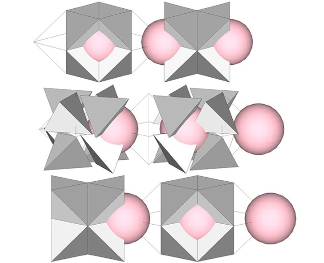
In previous posts, I’ve suggested that the jitterbug transformation may be associated with the migration of nuclei. The radially close-packed spheres of the isotropic vector matrix divide naturally into clusters in the shape of cubes and vector equilibria (VEs). See Space-Filling Polyhedra as Close-Packed Spheres. In the following illustration I’ve replaced the sphere clusters with tetrahedra. The eight tetrahedra that share a common vertex at the center of the VE are rotated 90°, or “jitterbug”, so that their common vertex faces outward to form the eight points of the cube. If we add the nuclei into this model, it suggests a migration of nuclei between the two.
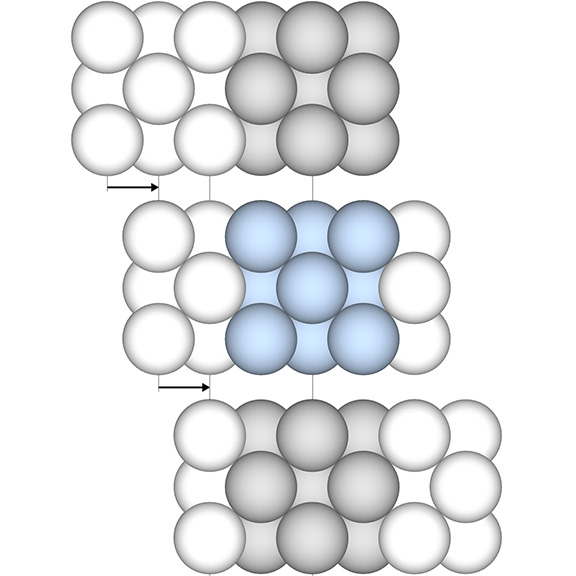
The effect of the jitterbug transformation may also be conceived as the shifting not only of nuclei but of all spheres comprising the isotropic vector matrix into their adjacent spaces. The natural axis for the transformation is that of the 3 Great Circles, the only axis on which every sphere is connected directly through the center of a space, i.e., a concave VE. (See: Spheres and Spaces, and Spaces and Spheres (Redux).)
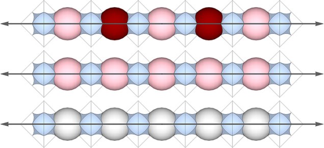
To see the outcome of the transformation, we need only shift our perspective—or hold our perspective constant while the matrix makes a lateral shift—left, right, up, down, in, or out—the distance of √2×r, where r is the radius of the sphere. In the illustration below we see a cube (blue) occupying the space previously occupied by a VE (gray), and then a VE (gray) again.
The identification of any single nucleus will have the effect of defining every other sphere in the isotropic vector matrix (see Formation and Distribution of Nuclei in Radial Close-Packing of Spheres). Nuclei are defined by their 12-sphere shells, and the remaining spheres (those that are neither a nucleus nor a sphere in a nucleus’s shell) are categorized as nuclear voids, i.e., nuclei whose shells consist entirely of spheres from the shells of their surrounding nuclei. (See Categories of Spheres in the Isotropic Vector Matrix: Nuclei, F1 Shells, and “Nuclear Voids”.) Implicit in the identification of any given sphere as a nucleus is the categorization of every other sphere; identifying a nucleus effectively “crystalizes” the matrix. Crystal lattices and networks are famously dull; the part tells the story of the whole. It is the jitterbug that makes it interesting.
As I said above, radially close-packed spheres divide naturally into vector equilibria and cubes, and we may think of one becoming the other in the jitterbug. In a “crystalized” matrix, we find three variations of each, i.e, three unique VEs and three unique cubes, each with a unique arrangement of the three categories of sphere. These I’m calling “blinkers,” borrowing from the lexicon of the legendary Game of Life which was developed by mathematician John Horton Conway in 1970.
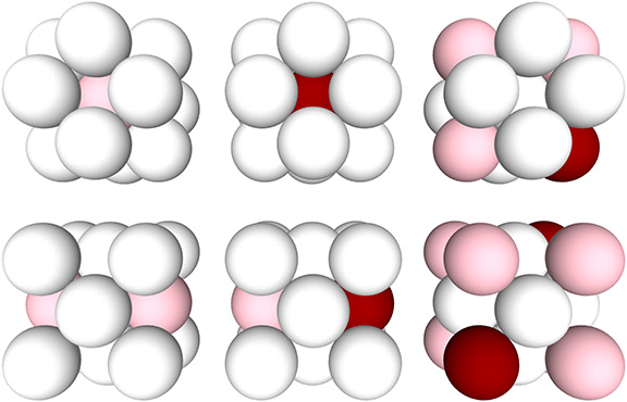
As the matrix jitterbugs, one cube or VE will be replaced with another—different, or the same rotated from its original orientation. They will appear to blink, flash, rotate, and oscillate as spheres are replaced by spaces and the spaces are replaced, again, by spheres. The jitterbug, in effect, can generate an infinite number of patterns that are replicated and regenerated throughout the matrix. In effect, the dull crystal is made into a kind of neural network by this interpretation of the jitterbug transformation.
