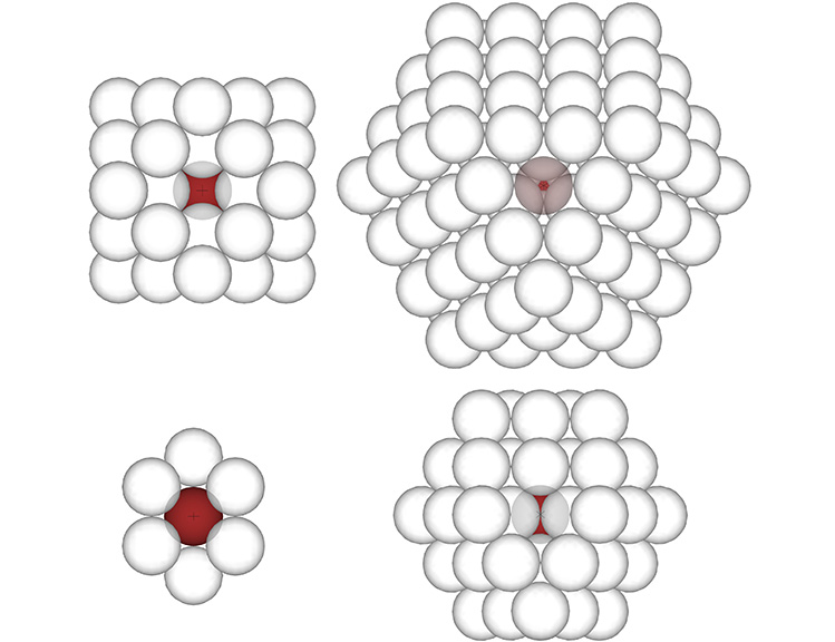
“The first layer consists of 12 spheres tangentially surrounding a nuclear sphere; the second omnisurrounding tangential layer consists of 42 spheres; the third 92, and the order of successively enclosing layers will be 162 spheres, 252 spheres, and so forth. Each layer has an excess of two diametrically positioned spheres which describe the successive poles of the 25 alternative neutral axes of spin of the nuclear group.”
— R. Buckminster Fuller, Synergetics, 222.23

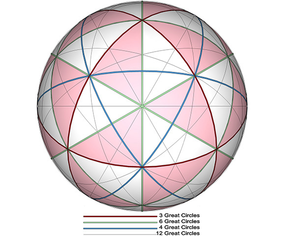
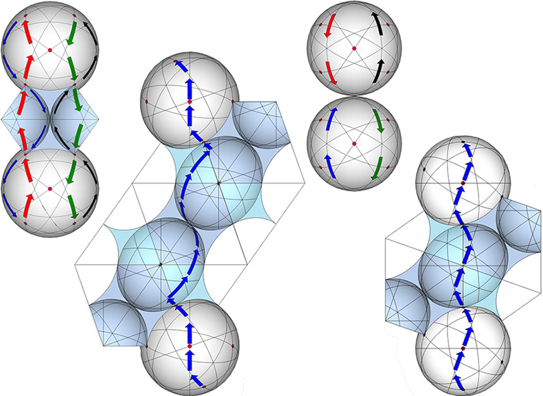
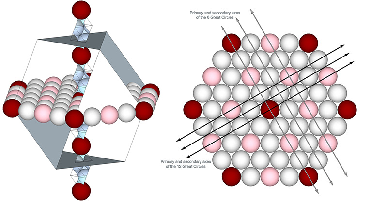
The four sets of 3, 4, 6, and 12 axes that define the 25 great circles of the vector equilibrium also comprise all line-of-sight connections between spheres radially close-packed in the isotropic vector matrix. That is, each axis proceeds directly, without deviation, through interstitial space from one sphere center to the next. This may be made more clear with the following illustration.

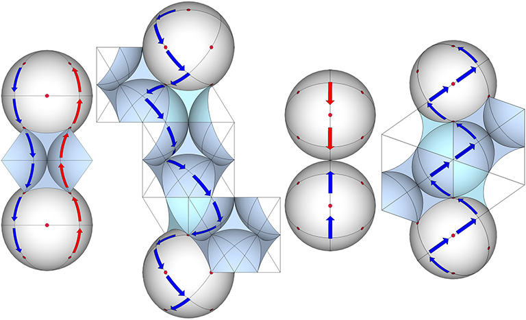
In the above illustration,

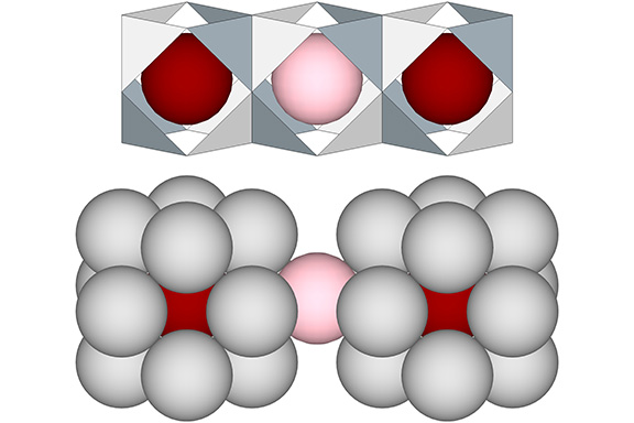
• The axis for the 3 great circles (top left) connects the semi-transparent sphere in the F2 layer with the nucleus (red), having passed through interstitial space in the F1 layer. Note that this is the only axis that provides a direct connection between nuclei and nuclear voids (see Categories of Spheres in the Isotropic Vector Matrix: Nuclei, F1 Shells, and “Nuclear Voids”). The semi-transparent sphere in the F2 layer will be surrounded by the F1 shells of its surrounding nuclei, and therefore qualifies as a nuclear void.
• The axis of the 4 great circles (top right) connects the semi-transparent sphere in the F3 layer with the nucleus (red) after having passed through interstitial space in both the F2 and F1 layers. Note that this is the only axis that provides a direct connection between nuclei; the semi-transparent sphere in the F3 layer will have its own layer of 12 spheres, and therefore qualifies as a nucleus.
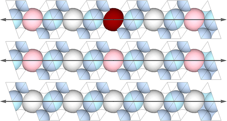
• The axis of the 6 great circles (bottom left) is unique in that it forms an unbroken chain of spheres in direct contact with one another. The semi-transparent sphere in the F1 shell is in direct contact with the nucleus.
• The axis of the 12 great circles (bottom right) connects the semi-transparent sphere in the F2 layer with the nucleus after having passed through what Fuller calls the “kissing point”, i.e., the point of contact between two spheres in the F1 layer.

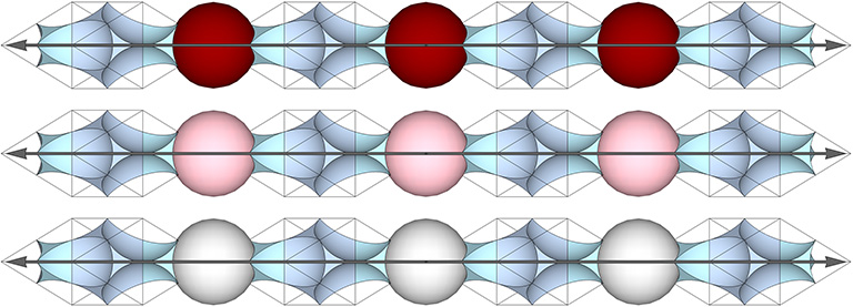
Set of 3 Great Circles of the VE

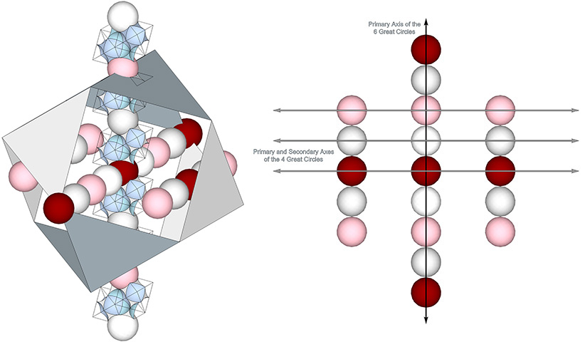
The axes of the 3 great circles pass through the centers of opposing square faces of the VE. Its primary axis connects nuclei in every fourth layer. Their great circle planes are in alignment with the three unique axes for the 3 Great Circles, and two of the three unique axes for the 6 Great Circles.

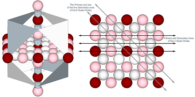
The axes pass alternately through a space (concave VE) and a sphere (convex VE). On the primary axes, the spheres alternate between nuclei (shown in red) and nuclear voids (pink). On the two secondary axes (those that do not pass through a nuclear sphere), the spheres are either all nuclear voids (pink) or spheres that occupy the F1 shells of nuclei. Shell spheres are shown in white. (See: Categories of Spheres in the Isotropic Vector Matrix: Nuclei, F1 Shells, and “Nuclear Voids”.)

Set of 4 Great Circles of the VE

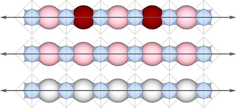
The axes of the 4 great circles pass through the centers of opposing triangular faces of the VE. Its primary axis connects nuclei in every 3rd layer. Their great circle planes are in alignment with the three unique axes for the sets 6 and 12 Great Circles.

The primary axis joins nuclei. The secondary axes join nuclear voids or shell spheres. Between each sphere on the axes is interstitial space consisting of a space (concave VE) flanked by one positive and one negative interstice (concave octahedra). See: Spheres and Spaces, and; Spaces and Spheres (Redux).

The axis of the set of four great circles is unique in that no single geodesic path directly joins the spheres along the axis. See Inter-Sphere Connections via the 25 Great Circles of the VE.

Set of 6 Great Circles of the VE

The axes of the 6 Great Circles pass through opposing vertices of the VE. Its primary axis connects nuclei in every fourth layer. Their great circle planes are in alignment with the three unique axes of the 4 Great Circles, the primary axis and and one secondary axis of the 3 great circles, and the primary axis of the 6 and 12 Great Circles.

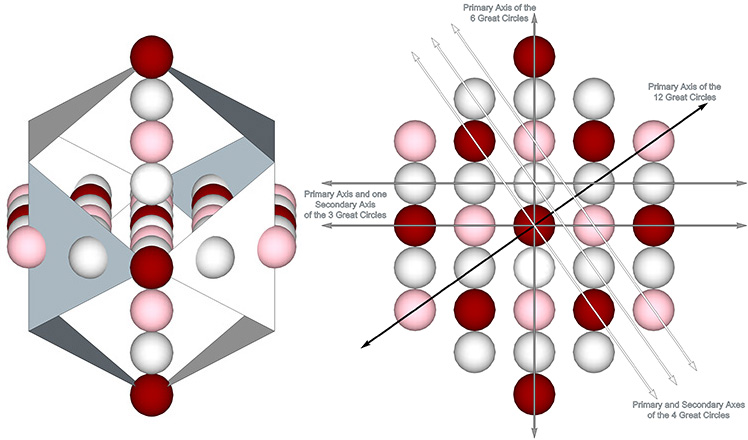
The primary axis joins nuclei and nuclear voids between each of which is a shell sphere. One secondary axes joins nuclear voids each separated by a shell sphere, and the other secondary axis forms an unbroken chain of shell spheres.

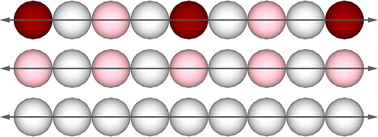
Set of 12 Great Circles of the VE

The axes of the 12 Great Circles pass through the centers of opposing edges of the VE. Its primary axis connects nuclei in every fifth layer. Their great-circle planes are in alignment with the three unique axes of the 4 Great Circles, and the primary axis of the 6 Great Circles.

Primary and secondary axes of the 12 great circles follow the same pattern as the axes of the 6 great circles, but with all all spheres separated by interstitial space.

Knowing how the three categories of spheres are distributed along the primary axes should enable us to count the total number of nuclei in each shell of the vector equilibrium. The primary axes for the sets of 3 and 6 Great Circles pass through a nucleus with every fourth shell. The primary axis for the Set of 4 Great Circles passes through a nucleus with every third shell And, the primary axes of the set of 12 Great Circles pass through a nucleus with every eighth shell. It follows that only those shells which are multiples of 3, 4 and 8 contain nuclei. The F1, F2, and F5 shells, for example, have none. We also know that nuclei are evenly distributed on a grid of rhombic dodecahedra (see Formation and Distribution of Nuclei in Radial Close-Packing of Spheres), and that the shell growth formula for the rhombic dodecahedron is 12F²+2 (see Concentric Sphere Shell Growth Rates). If anyone knows, or is able to derive the formula, please share.

“Whereas each of the 25 great circles of the vector equilibrium go through the 12 vertexes at least twice; and whereas the 12 vertexes are the only points of inter-tangency of symmetric, unit-radius spheres, one with the other, in closest packing of spheres; and inasmuch as we find that energy charges always follow the convex surfaces of systems; and inasmuch as the great circles represent the most economical, the shortest distance between points on spheres; and inasmuch as we find that energy always takes the most economical route; therefore, it is perfectly clear that energy charges passing through an aggregate of closest-packed spheres, from one to another, could and would employ only the 25 great circles as the great circle railroad tracks between the points of tangency of the spheres, ergo, between points in Universe. We can say, then, that the 25 great circles of the vector equilibrium represent all the possible railroad tracks of shortest energy travel through closest-packed spheres or atoms.”
—R. Buckminster Fuller, Synergetics, 458.01

Fuller proposed that the 25 great circles of the vector equilibrium account for all the routes by which energy is transmitted between spheres in the isotropic vector matrix. Or, to put it more dramatically, the great circles defined by the four sets of 3, 4, 6 and 12 spin axes of the VE represent all possible tracks of shortest energy travel between points in the universe.

See: Great Circles: The 25 Great Circles of the Vector Equilibrium (VE), and; The 25 Great Circles of the VE (new illustrations)

All great circle trajectories may be reduced to combinations of the shortest-distance paths for each set of great circles connecting adjacent spheres on each of the four axes. (See Distribution of Radially Close-Packed Spheres on the 25 Axes and Great Circle Planes of the Vector Equilibrium.)

The Set of 3 Great Circles

The great circles in the set of 3 are defined by spin axes running through the centers of opposing square faces of the VE. Each great circle passes through four vertices and therefore has four opportunities with each 360° circuit to connect to an adjacent sphere.

• On the axis of the 3 great circles, the set of 3 reveals four equally efficient paths, two of which are shown below (left).
• On the axis of the 4 great circles, the set of 3 reveals six equally efficient paths, one of which is shown in below (left middle).
• All of the great circle sets connect spheres on the axis of the 6 great circles with equal efficiency, differing only in the number of alternate paths; the set of 3 (right middle), reveals two.
• On the axis of the 12 great circles, the set of 3 reveals two equally efficient paths, one of which is shown below (right).

The Set of 4 Great Circles

The great circles in the set of 4 are defined by spin axes running through opposing triangular faces of the vector equilibrium (VE). Each great circle passes through six vertices and therefore has six opportunities with each 360° circuit to connect with an adjacent sphere.

• On the axis of the 3 great circles (top), the set of 4 reveals eight equally-efficient helical routes that complete a cycle every other sphere.
• On the axis of the 4 great circles (middle top), the set of 4 reveals eight equally-efficient helical routes the complete a cycle every fourth sphere.
• On the axis of the 6 great circles (middle bottom), the set of 4 reveals four equally-efficient routes between spheres.
• On the axis of the 12 great circles (bottom), the set of 4 reveals two equally-efficient routes between spheres.

The Set of 6 Great Circles

The great circles in the set of 6 are defined by spin axes running through opposing vertices of the vector equilibrium (VE). Each great circle passes through two diametrically opposed vertices.

• On the axis of the 3 great circles, the set of 6 (left) reveals 4 equally-efficient routes between spheres.
• On the axis of the 4 great circles, the set of of 6 (middle left) reveals a branching network of at least 36 equally-efficient paths.
• On the axis of the set of 6 great circles, the set of 6 (middle right) reveals two equally-efficient paths between spheres.
• On the axis of the 12 great circles, the set of 6 (right) reveals two equally-efficient paths between spheres.

The Set of 12 Great Circles

The great circles in the set of 12 are defined by spin axes running through the midpoints of opposing edges of the vector equilibrium (VE). As with the set of 6, each great circle in the set of 3 passes through two diametrically opposed vertices.

• On the axis of the set of 3 great circles (left), the set of 12 reveals eight equally-efficient routes between spheres.
• On the axis of the 4 great circles (middle left), the set of 12 reveals four equally-efficient paths, one of which is shown.
• On the axis of the set of 6 great circles (middle right), the set of 12 reveals four equally-efficient paths.
• On the axis of the set of 12 great great circles (right), the set of 12 reveals two equally-efficient paths, one of which is shown.

When modeling the distribution of nuclei in the isostropic vector matrix, I distinguish between the nuclei and the 12-sphere shells that isolate and define them. These nuclear domains, each consisting of one nuclear sphere and a 12-sphere shell, defines the vector equilibrium, or VE.

Nuclei are distributed throughout the isotropic vector matrix at the centers and vertices of close-packed rhombic dodecahedra whose edges align with the primary axes of of the vector equilibrium’s 4 great circles. See: Formation and Distribution of Nuclei in Radial Close-Packing of Spheres; and Great Circles: The 25 Great Circles of the Vector Equilibrium (VE); The 25 Great Circles of the VE (new illustrations); and Distribution of Radially Close-Packed Spheres on the 25 Axes and Great Circle Planes of the Vector Equilibrium.

Nuclei and their shells do not close-pack to fill all-space. Between these nuclear clusters are gaps which combine for form holes that run laterally through the isotropic vector matrix.

The spheres that fill these voids can be isolated to show that they all lie on a cubic grid which follows the square-face diagonals of close-packed F2 VEs.

I refer to these as “nuclear voids” because, like the nuclei, each occupies the center of a VE, but unlike the nuclei, they do not have their own 12-sphere shells. Rather, every sphere in direct contact with a “nuclear void” is uniquely identified with the shell of one of its neighboring nuclei.