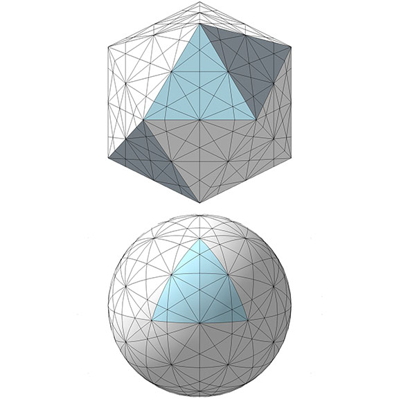
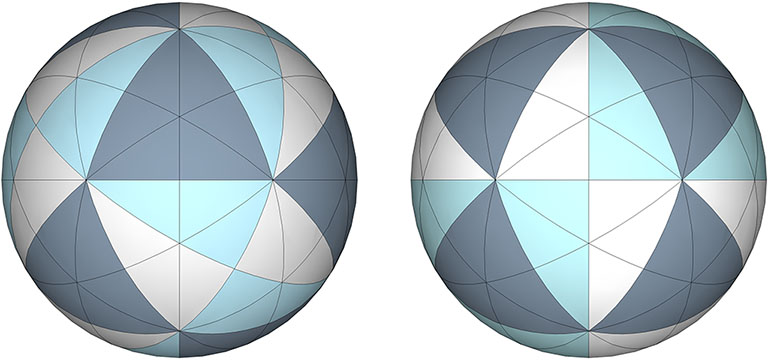
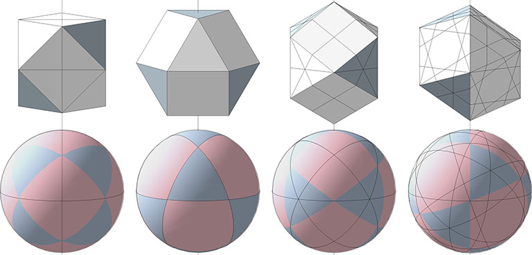
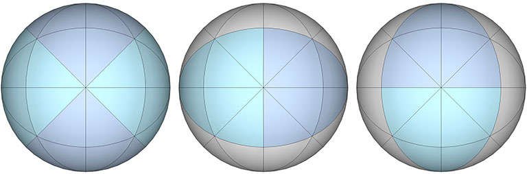
The figure below illustrates the full set of 31 great circles described by rotations about the regular icosahedron’s axes of symmetry.
The 31 great circles of the icosahedron as projected onto the planar icosahedron (top) and sphere (bottom).
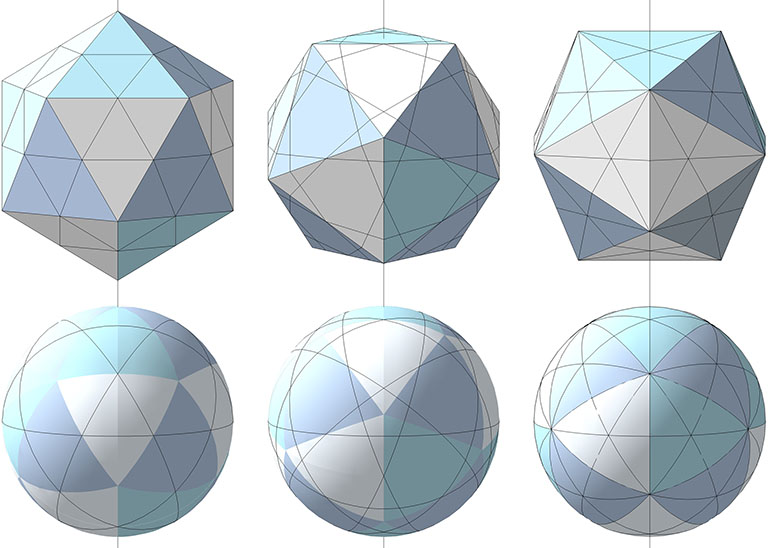
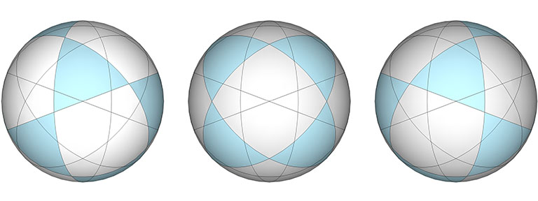
The 31 great circles are divided into three sets according to their spin axes. Axes running through diametrically opposing vertices generate the set of 6 great circles. Axes running through opposite faces generate the set of 10 great circles. And axes running through the midpoints of diametrically opposing edges generate the set of 15 great circles.
Left to right: the set of 6 great circles on axes running though opposing vertices; the set of 10 great circles on axes running through the centers opposing faces, and; the set of 15 great circles on axes running though he midpoints of opposing edges.
6 Great Circles
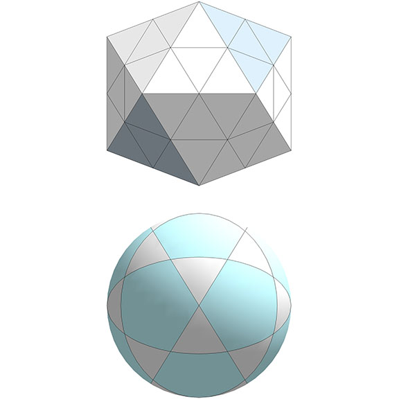
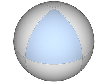
The set of 6 great circles circumscribes the equators of the six spin axes that pass through the icosahedron’s opposing vertices, and together they disclose the spherical icosidodecahedron.
The set of 6 great circles of the icosahedron disclose the spherical icosidodecahedron.
15 Great Circles
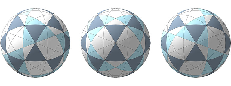
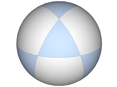
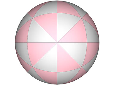
The set of 15 great circles disclose the two orientations of the spherical octahedron, the spherical icosahedron, pentagonal dodecahedron, rhombic triacontahedron, and the 120 basic disequilibrium LCD triangles.
The set of 15 great circles of the icosahedron disclose two orientations of the spherical octahedron (left); the spherical icosahedron (top middle); the rhombic triacontahedron (bottom middle); the 120 basic disequilibrium LCD triangles (top right); and the pentagonal dodecahedron (bottom right).
The same spherical icosahedron is symmetrically aligned with both orientations of the spherical octahedron. See also: Icosahedron Inside Octahedron.
Both orientations of the spherical octahedron align symmetrically with the same spherical icosahedron disclosed by the 15 great circles of the icosahedron.
10 Great Circles
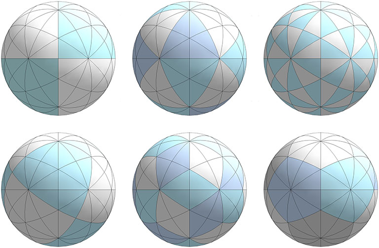
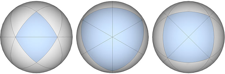
The set of 10 great circles discloses three orientations of the spherical vector equilibrium (VE).
Three orientations of the vector equilibrium (VE) as disclosed by the 10 great circles of the icosahedron.
The same spherical icosidodecahedron (generated from the six great circles) is symmetrically aligned with all orientations of the spherical vector equilibrium (VE).
All three orientations of the VE as disclosed by the 10 great circles of the icosahedron are symmetrically aligned with the same icosidodecahedron disclosed by the 6 great circles.
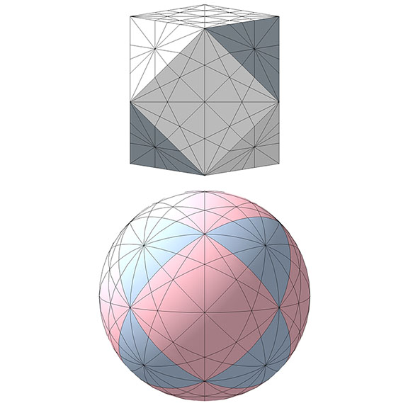
The figure below illustrates the full set of great circles in the context of the vector equilibrium (VE), both the planar VE (top), and spherical VE (bottom). Note that twelve great circles converge, cross, or are deflected at each of the twelve vertices, and at the centers of each triangular face.
The 25 great circles of the vector equilibrium (VE)
The 25 great circles are divided into four sets according to their spin axes. Axes running through opposite square faces generate the set of 3 great circles. Axes running through the centers of opposite triangular faces generate the set of 4 great circles. Axes running through diametrically opposing vertices generate the set of 6 great circles. And axes running through the midpoints of diametrically opposing edges generate the set of 12 great circles.
Left to right: Set of 3 great circles on axes through opposing square faces; Set of 4 great circles on axes running through opposing triangular faces; Set of 6 great circles on axes running through opposing vertices; Set of 12 great circles with axes running through opposing edges.
3 Great Circles
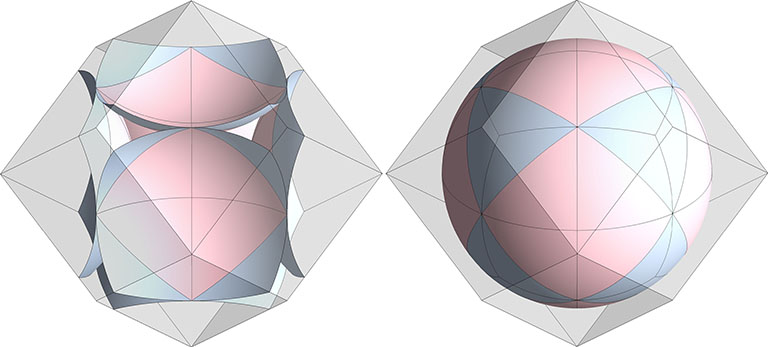
The set of 3 great circles discloses the spherical octahedron.
The spherical octahedron disclosed from the set 3 great circles, with one face highlighted.
4 Great Circles
The set of 4 great circles discloses the spherical vector equilibrium (VE).
The spherical VE disclosed from the set of 4 great circles, with its triangular faces highlighted.
6 Great Circles
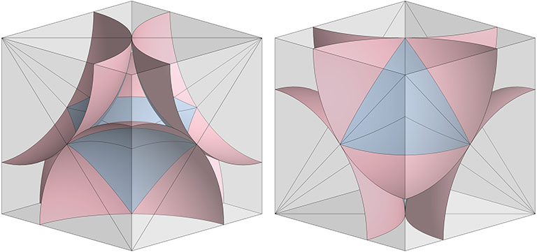
The six great circles disclose the spherical rhombic dodecahedron, the spherical tetrahedron (both positive and negative), and the spherical cube.
The set of 6 great circles disclosing, left to right: the spherical rhombic dodecahedron; the spherical tetrahedron, and; the spherical cube, each with one face highlighted.
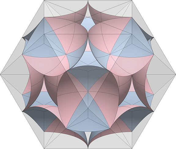
The six great circles complement the three great circles to disclose three additional octahedra.
The sets of 3 and 6 great circles disclose three additional spherical octahedron.
The sets of 3 and 6 great circles of the VE disclose the 48 basic equilibrium LCD triangles.
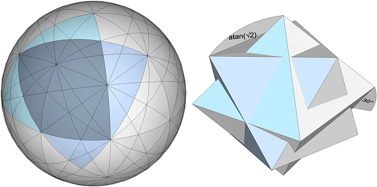
12 Great Circles
The twelve great circles of VE do not appear to disclose, by themselves, any of the regular polyhedra. However, in combination with the 4 and 6 great circle sets, the 12 great circles do disclose an alternate spherical regular octahedron that is curiously askew from the others, rotated 30° on the z axis, and atan(√2) on the y axis.
The 4, 6, and 12 great circles of the VE each contribute one edge to disclose a spherical octahedron whose axes are curiously skewed from all the other polyhedra the 25 great circles of the VE disclose.
“The closest-packed symmetry of uniradius spheres is the mathematical limit case that inadvertently captures all the previously unidentifiable otherness of Universe whose inscrutability we call space. The closest-packed symmetry of uniradius spheres permits the symmetrically discrete differentiation into the individually isolated domains as sensorially comprehensible concave octahedra and concave vector equilibria, which exactly and complementingly intersperse eternally the convex “individualizable phase” of comprehensibility as closest-packed spheres and their exact, individually proportioned, concave-in-betweenness domains as both closest packed around a nuclear uniradius sphere or as closest packed around a nucleus-free prime volume domain.” —R. Buckminster Fuller, Synergetics, 1006.12
Spaces, like spheres, have surfaces. The interstitial model of the isotropic vector matrix (IVM) makes evident that it is the sphere’s surfaces (both its convex and its concave surfaces) that matter. Electric charge is carried on the surface of the conductor. Molecular biology is all about the lock and key system of protein surfaces and shapes. The surface of the “space” in the isotropic vector matrix is a continuity broken only be the seams at the interface of the concave “spaces” and “interstices” (see below). These seams align with the four great circles of the vector equilibrium (VE), and describe the most efficient paths between the points of contact with adjacent spheres. See also: Anatomy of a Sphere.
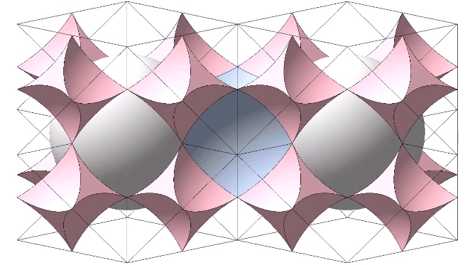
The figure below shows the exact correlation between two models of the isotropic vector matrix, a correspondence that Fuller attempted to describe in the excerpt I’ve quoted above.
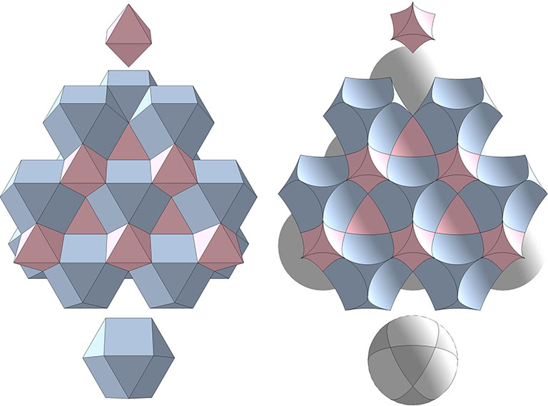
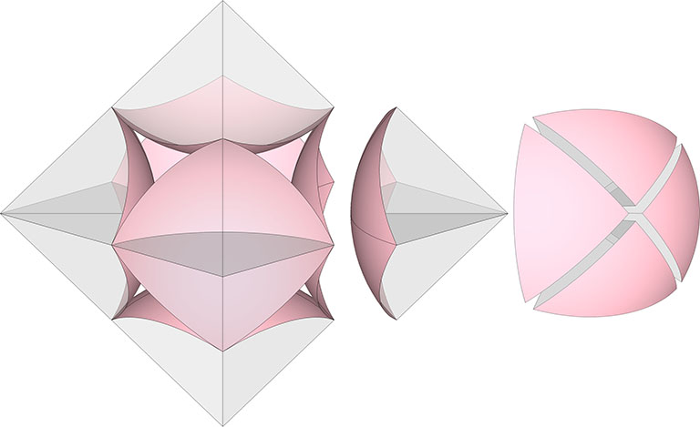
Space Filling of Octahedron and Vector Equilibrium: The packing of concave octahedra, concave vector equilibria, and spherical vector equilibria corresponds exactly to the space filling of planar octahedra and planar vector equilibria. Exactly half of the planar vector equilibria become convex; the other half and all of the planar octahedra become concave.
Though the VEs (blue) and octahedra (pink) on the left align with the spaces (blue) and interstices (pink) on the right, close inspection of the above models reveals a key difference. The model on the left does not distinguish between spheres and spaces. While on the right the difference is obvious, on the left both spheres and spaces are represented by identical VEs. The ambiguity is apt: In the isotropic vector matrix, there is a one-to-one identity between the spheres and spaces; one is simply the other turned inside out.
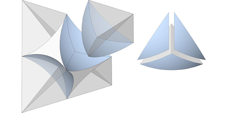
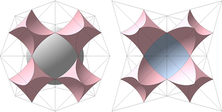
The model on the right is what I’m calling the interstitial model of the isotropic vector matrix. It consists of concave vector equilibrium (VE) spaces and concave octahedron interstices. The concave VE is the shape of the void at the center of six close-packed spheres defining the octahedron. The concave octahedron is the shape of the void at the center of four close-packed spheres defining the tetrahedron.
Concave VE (“space”)
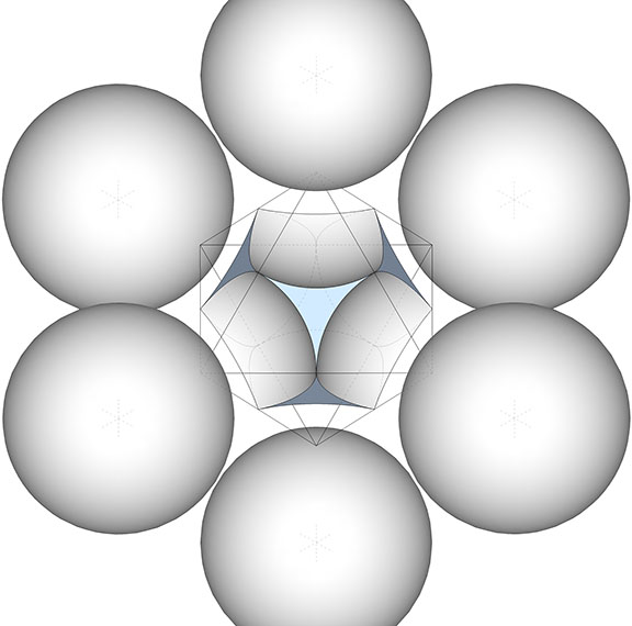
Because it occupies the space in the isotropic vector matrix that is replaced by a sphere in the jitterbug transformation, I reserve the term “space” for the concave VE at the common center of the six close-packed spheres of the regular octahedron.
The void at the center of the six close-packed spheres centered on the vertices of the regular octahedron has the shape of a concave vector equilibrium (VE). In the jitterbug transformation, this “space” is turned inside-out to define the spherical VE or “sphere.”
Concave Octahedron (“interstice”)
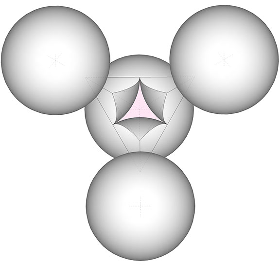
The void at the center of four close-packed spheres has the shape of a concave octahedron which I call the “interstice” to distinguish it from the “space” referred to above. The interstices maintain both their shape and position during the jitterbug transformation, while their 90° rotations articulate the sphere-to-space oscillations described below.
The void at the center of the four spheres centered on the vertices of the regular tetrahedron has the shape of a concave octahedron. These “interstices” are rotated 90° to alternately define the spheres and spaces that exchange places in the jitterbug transformation.
Spherical Domains
The polyhedra of the isotropic vector matrix divide the spheres into rational sections which, when added together, constitute the polyhedron’s spherical domain. Fuller thought this rationality was sufficient to eliminate pi (π) from his geometry. He’d already shown that the volumes of most polyhedra were rational if instead of the cube we used the regular tetrahedron as the unit volume. And if we replaced the irrational volume of the sphere with the rational sections carved from the rational polyhedra, pi was irrelevant.
Rhombic Dodecahedron
144 quanta modules
1 spherical domain
Vector Equilibrium (VE)
480 quanta modules
3.40 spherical domains
Cube
72 quanta modules
1/2 spherical domain
Octahedron
96 quanta modules
3/5 spherical domain
Tetrahedron
24 quanta modules
1/5 spherical domain
Octahedron
The six spheres at the vertices of the octahedron define the concave vector equilibrium space at its center. The planar facets of each vertex carve a 1/10 section from its sphere. The 1/10 section is further subdivided to form the four 1/40 sections used in the spherical domain calculations. The total spherical domain of the planar octahedron is 3/5.
The planar octahedron cuts 1/10 sections from each of its six spheres, for a total spherical domain of 3/5. Each of these 1/10 sections is further subdivided into four 1/40 sections which are used to calculate the spherical domains of the remaining polyhedra.
Tetrahedron
The four spheres at the vertices of the tetrahedron define the concave octahedron interstice at its center. The planar facets of each vertex carve a 1/20 section from its sphere. The 1/20 section is further divided to form the three 1/60 sections used in the spherical domain calculations. The total spherical domain of the planar tetrahedron is 1/5.
The planar tetrahedron cuts 1/20 sections from each of its four spheres, for a total spherical domain of 1/5. Each of these 1/20 sections is further subdivided into three 1/60 sections which are used to calculate the spherical domains of the remaining polyhedra.
Rhombic Dodecahedron
There are two rhombic dodecahedra in the isotropic vector matrix—one with a space at its center, and one with a sphere. For the rhombic dodecahedron with a space at its center, each of the six acute vertices define the center of a sphere from which the planar facets of each carve a 1/6 section. Both of the planar rhombic dodecahedra contain precisely one spherical domain.
Note that one is made from the other by reversing the 1/6 sections so that their peaks point either inward to define the sphere, or outward to define the space.
The planar rhombic dodecahedron on the left cuts 1/6 sections from each of the six spheres centered on its six acute vertices, for a total spherical domain of 1, the same spherical domain of the rhombic dodecahedron on the right, where the 1/6 sections have been rotated 180° so that their convex faces are pointing outward.
Cube
There are two cubes in the isotropic vector matrix, one a 90° rotation of the other. Their rotation comprises the jitterbug transformation and the exchange between spheres and spaces. Four of its eight vertices each define the center of a sphere from which the planar facets of each carve a 1/8 section. The planar cube contains precisely 1/2 spherical domain.
The planar cube carves a 1/8 section from the spheres centered on four of its eight vertices, for a total spherical domain of 1/2. The cube on the right is a 90° rotation of the cube on the left. This rotation accounts for the sphere-to-space oscillations of the isotropic vector matrix in the jitterbug transformation.
Vector Equilibrium (VE)
The twelve vertices of the VE each define the center of a sphere from which the planar facets carve a 1/5 section. These plus the nuclear sphere add to a total of 3.4 spherical domains.
The planar vector equilibrium (VE) carves 1/5 sections from each of the twelve spheres centered on its vertices. These plus the nuclear sphere total add to 3.4 spherical domains.
Ratio of Spheres to Spaces in the Isotropic Vector Matrix
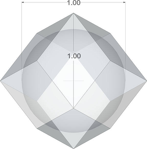
While the sphere-to-space ratio differs for the polyhedra, when the isotropic vector matrix is considered as a whole the ratio approaches that of the rhombic dodecahedron; rhombic dodecahedra close pack exactly as spheres close pack, and the rhombic dodecahedron constitutes one spherical domain.
The volume of the unit-diameter sphere is π√2 tetrahedra and the volume of the rhombic dodecahedron which contains that sphere is six unit tetrahedra. So, the sphere-to-space ratio is (π√2)/(6 – π√2), or ≈ 2.853275. Fuller wanted this number to be rational. It is not.
The domain of the radially close-packed unit-diameter sphere is a rhombic dodecahedron whose in-sphere radius and long face diagonal are of unit length, and whose tetrahedral volume is exactly 6.
Sphere-to-Space and Space-to-Sphere Oscillation of the Jitterbug
The interstitial model provides the most literal interpretation of the space-to-sphere oscillations of the jitterbug. The tetrahedron’s polarity reversal is accomplished by a 90° rotation of the concave octahedron interstices which alternately disclose the nuclear sphere, on the left in the illustration below, and the nuclear space, on the right:
The concave octahedron interstices are rotated 90° to alternately disclose the nuclear sphere at the center of the vector equilibrium (left), and the nuclear space at the center of the octahedron (right).
The 90° rotation of the concave octahedra interstices at the centers of positive and negative tetrahedra account for the sphere-space oscillations of the jitterbug transformation.