Note: For instructions on how to construct the Weaire-Phelan structure, see my post: Construction Method for the Pyritohedron and Tetrakaidecahedron of the Weaire-Phelan Structure.

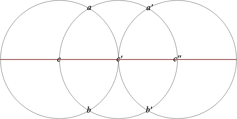
Pyritohedra and tetrakaidecahedra close pack to constitute the Weaire-Phelan structure (or Weaire-Phelan “matrix” as I prefer to call it, and, when dimensioned appropriately, align precisely with the distribution of nuclei in the isotropic vector matrix. The unit vector (d in the illustration below) is identical with the unit vector (sphere diameter) of the isotropic vector matrix.

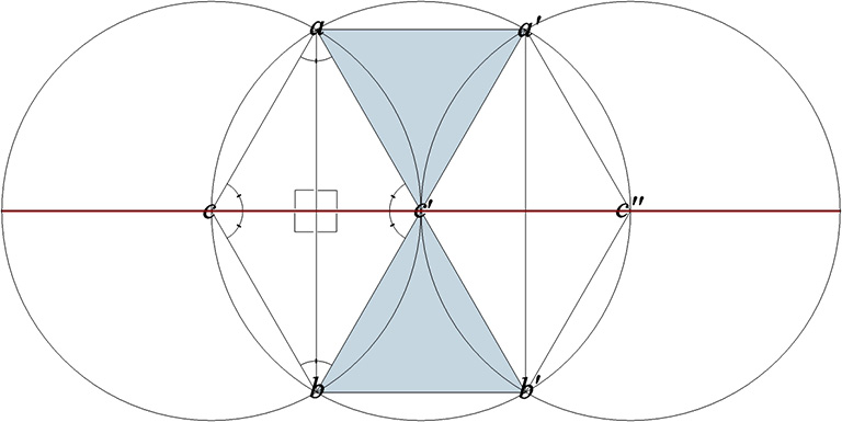
The pyritohedron and, presumably, the tetrakaidecahedron have identical rational volumes in both cubic and tetrahedral units of measure. For the cubic volume, we take the long edge of the pentagonal face as the unit length (a in the illustrations). For the tetrahedral volume, we take the diameter of the sphere as the unit length (d in the illustrations).

When we measure the angles, edge lengths, and radii of the pyritohedron, the numbers do not inspire confidence. It would seem unlikely that so many irrational numbers could possibly result in a rational, whole-number volume. But they do.

a = long edge or base of pentagonal face
d = diameter of sphere*
d = a × ³√4 × √2/2
a = d × ³(√2/2) = (d√2)/(³√4) = d√2 × ³√(1/4)

*d is identical with the unit vector of the isotropic vector matrix. In the Weaire-Phelan matrix, it aligns with the height vectors connecting the base with the peak of the smaller of the two pentagonal faces of the tetrakaidecahedron, and to the radial vectors connecting the height vector’s endpoints (see illustration below).

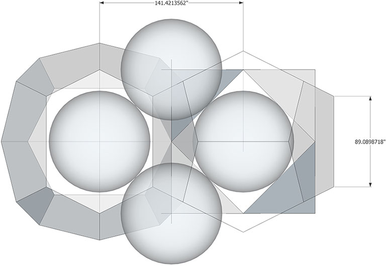
The long edge of the pyritohedron’s pentagonal face, a, (which, when taken as unit length results in a cubic volume for the pyritohedron of 4a³) seems to be related to the diameter of the sphere, d, by ³(√2/2) or about 0.890898718. I don’t have a geometric proof to account for the appearance of this third root, but the number seems to work to at least 7 decimal places in my computer models, and the irrational roots cancel out perfectly in the volume calculations to produce the rational result of 24d³ for the tetrahedral volume.

Pyritohedron specifications:

• 12 irregular pentagonal faces, 20 vertices, 30 edges
• Face angles:
  • atan(2√5) + atan(√5/4) ≈ 106.6015496°
  • atan(√5/10)+90° ≈ 102.6043826°
  • 2atan(4√5/5) ≈ 121.588136°
• Dihedral angle: 2atan(2) ≈ 126.8698976°
• Volume (in tetrahedra): 24a³√2
• Volume (in tetrahedra): 24d³
• Cubic volume: 4a³
• Cubic volume: 2d³√2
• Quanta modules: 576 modules, types unknown*
• Surface area (in equilateral triangles): 8a²√15
• Surface area (in squares): 6a²√5
• In-sphere radius: 2a/√5
• Mid-sphere radius (center to mid-long-edge): a
• Circum-sphere radius: a√5/2

*It should be possible to construct the pyritohedron from quanta modules, but may involve one or more variants of those quanta modules already described by by Fuller.

The image below shows my computer model with the calculated dimensions accurate to 7 decimal places.

Geodesic polyhedra are convex polyhedra consisting of triangles, and include the spherical polyhedra generated by subdividing the faces of a tetrahedron, octahedron, or icosahedron into smaller triangles and projecting their crossings out to the underlying polyhedron’s circumsphere radius. Those based on the icosahedron are related to but not necessarily aligned with the 31 great circles of the icosahedron from which their name seems to have originated. The name “geodesic” refers to Fuller’s early conviction that only a triangular latticework of geodesic lines would serve to distribute local stresses evenly throughout the system he patented under the name “Geodesic Dome” in 1954. As the domes evolved into the systems of mostly partial great circles and lesser circles described here, the term “geodesic polyhedra” preserved the memory of that earlier conviction.

Geodesic polyhedra are defined by the equilateral triangles of the primary face (i.e., the face of the underlying tetrahedron, octahedron, or icosahedron) laid out on a 60° grid so that their vertices always align with grid crossings. This produces three classes of tiling or tessellation. The edges of the primary triangular face in Class 1 are parallel to the grid lines. The edges in Class 2 are perpendicular to the grid lines. Those in Class 3 are neither parallel nor perpendicular to the grid lines.

The frequency of each class is given by two numbers (b,c) representing the number of triangular modules along the grid lines connecting adjacent vertices. The general formula for the area, or the number of triangular modules that subdivide the primary face, is given by:

Area (T) = b² + c² + (b×c)

For Class 1, b is the edge length of the primary face; so, c is always 0 and the formula reduces to b². For Class 2, b = c, so the formula can be reduced to 3b².

Class 1 Geodesics

Class 1 geodesics subdivide the primary face with lines parallel to the edges.

Class 2 Geodesics

Class 2 geodesics subdivide the primary face with lines perpendicular to the edges.

Class 3 Geodesics

Class 3 geodesics subdivide the face with lines that are askew to the edges, neither parallel no perpendicular.

All of the geodesic polyhedra above have as their base the regular icosahedron. Being the most spherical, the icosahedron generates the most uniform tessellations. But the geodesic polyhedra may also be generated using the tetrahedron as their base, as in the following examples:

And they may also be generated using the octahedron as their base, as in these examples:

The spherical tensegrities, whether based on the tetrahedron, octahedron, or icosahedron, have the shape of Goldberg polyhedra, the duals of geodesic polyhedra. Fuller held that all of his geodesic domes were, structurally, tensegrities. But then, any self-supporting structure can be described as a tensegrity. That is, all structural arrangements of vectors can be described as islands of compression in a continuous web of tension. Perhaps Fuller meant that his calculations were done on the spherical tensegrities, i.e., the tensor equilibrium phases of the tensegrity forms of the geodesic polyhedra. (See: Tensegrity, and; Tensegrity Equilibrium and Vector Equilibrium.) Many of Fuller’s domes do, in fact, have the appearance of Goldberg polyhedra. Fuller’s geodesic structures may be most accurately described as tensegrity composites incorporating both their spherical and polyhedron states.

An alternate construction of the 2F Class 1 geodesic polyhedron is achieved by reducing the the 120-strut tensegrity sphere to its polyhedron phase.

Composite tensegrities, incorporating the spherical (Goldberg) and polyhedron (geodesic) phases of two or more frequencies may be possible without one interfering with the other. These may be easier to construct and would no doubt have incredible strength.

“You can “draw a line” only on the surface of some system. All systems divide Universe into insideness and outsideness. Systems are finite. Validity favors neither one side of the line nor the other. Every time we draw a line operationally upon a system, it returns upon itself. The line always divides a whole system’s unit area surface into two areas, each equally valid as unit areas. Operational geometry invalidates all bias.”
—R. Buckminster Fuller, Synergetics, 811.04

All of Fuller’s geometry is “operational” in the sense that it is conveyed and verified by physical models. The operations of synergetics includes constructions of sticks and flexible connectors, quanta modules, struts and string, wire, elastic cord, paper disks, clusters of ping-pong balls, a list of materials and operations limited only by our imaginations. Science without models is like language without metaphor. In the absence of metaphor, language is merely encoded logic. And without models, Fuller argued, science is equally impoverished. We need metaphor to formulate and articulate as yet unidentified concepts, and models are the metaphors of science. (See: Model Making.)

By way of introducing his operational geometry, Fuller would recall the basic operations of Euclidean geometry. Anyone who’s been through grade school has probably been taught how to use a draftsman’s compass, a straight edge, and a pencil, to repeat the familiar operation by which to find the perpendicular to a line and to construct an equilateral triangle.

Begin by drawing a circle with the dividers of the compass tightened to a fixed radius. Next, with the straight edge, draw a line from its center (c) to the circle’s perimeter. Fix the compass on the point where the line crosses the circle’s perimeter (c’) and draw another circle. Repeat and draw a third circle centered at the point where the straight line crosses the perimeter of the second circle (c”).

Now you have three circles bisected by a straight line running through the the circle centers, c, c’, and c”. The second circle crosses the first at two points, a and b. The third circle crosses the second at two points, a’ and b’. Lines drawn from a to b, and from a’ to b’ are perpendicular to the line drawn between the circle centers. Finally, draw lines between adjacent points to create six equilateral triangles in the shape of a hexagon.

Fuller often argued that the key shortcoming of plane geometry is its failure to account for the surface on which its operations are performed. The surface is a tool, just like the dividers, the straight edge, and the stick we scratch the surface with.

With the surface in mind, Fuller re-imagined the above operations as follows:

Begin by scribing a sphere. Granted, it isn’t possible to “scribe a sphere.” But we can imagine the process and perform the remaining operations on the surface of the sphere whose radius we are assured is identical with the fixed distance between the dividers of our compass. Mark a center anywhere on the sphere’s surface and draw a circle using the same compass. Next, just as before, draw a straight line from the center (C) to a point on the circle’s perimeter. And, remembering that straight lines on curved surfaces are, by definition, geodesics, we can continue drawing the line until it returns to the circle’s center and divides the sphere into two equal halves. Next, center the compass on one of the two points where the line crosses the perimeter of the circle and draw a second circle. Repeat, as above, to draw a third circle.

Now, when we connect the points as before with straight-line geodesics, we find that we have drawn four great circles. We know, operationally, that the length of the chords between the points is identical with the the sphere’s radius.

We have inadvertently constructed the eight equilateral triangles and six square faces of the vector equilibrium (VE). If we connect the points with the sphere center we create the eight tetrahedra and six half-octahedra that form the core of the isotropic vector matrix. And we have done it all operationally, without any calculations, and using only a compass, straight edge, and pencil.

Fuller considered plane geometry to be a special case of the more general field of spherical trigonometry and topology. The Euclidean plane is a hemispheric section sliced through the middle of the sphere, and plane geometry is then the measurement of the chords whose central angles define the arcs of great circles drawn on the sphere’s surface.