Another way to visualize the difference between the two equilibrium phases of the jitterbug—tensegrity equilibrium (see Jessen Orthogonal Icosahedron and Tensor Equilibrium, and Tensegrity) and vector equilibrium (see Vector Equilibrium and the “VE”)—is to observe the path followed by the triangles’ vertices. In the case of the tensegrity model of the isotropic vector matrix, and if the tendons are assumed be elastic and the struts to be non-compressible, the path follows the edges of the cube in the which the triangle rotates. In the vector model, the triangle’s vertices follow an arc coincident with the cube’s orthogonal planes and are identical with cube’s vertices at the VE and octahedron phases.
In the model below, tensegrity equilibrium is represented by an elastic cord stretched between three rings attached to the cube’s edges. Given negligible friction between the rings and the edges, the cord will find its natural equilibrium in the position shown, coinciding the the Jessen Orthogonal Icosahedron, i.e., the shape of the unstressed 6-strut tensegrity sphere.
A loop of elastic cord stretched between three edges of a wireframe cube with frictionless rings will find its natural equilibrium in a position identical with the edges of Jessen orthogonal icosahedron and the tendons of the six-strut tensegrity sphere.
Elastic loops stretched between the edges of a cubic scaffold with frictionless rings describe the shape of the six-strut tensegrity sphere and Jessen orthogonal icosahedron.
Equilibrium in the vector model is represented in the illustration below by the pink spheres nestled in the valleys of the arcs followed by the vertices of the triangles’ triangles rotation in the jitterbug transformation—which coincides with the octahedron phase of the jitterbug. The instability of the de-nucleated VE (the removal its nucleus, or radial vectors, is what precipitates the jitterbug) is represented by the blue spheres when they are precariously perched at the peaks of the arcs.
Vector equilibrium modeled as dips in the arcs described triangle’s rotations in the jitterbug.
The third shell of radially close-packed, unit-radius spheres around a common nucleus consists of 92 spheres, a number that Buckminster Fuller did not consider coincidental. (See: Close-Packing of Spheres.) The Periodic Table of Elements, with its 92 stable elements ranging from hydrogen to uranium is after all the close packing of neutrons and protons. Also intriguing is the emergence, in the third shell, of eight new potential nuclei at the centers of the eight triangular faces.
Eight unique nuclei emerge in the third shell of radially close-packed spheres. The third shell contains 92 spheres, suggesting a correspondence to the number of stable atoms in the periodic table of elements.
If these eight spheres are added to the second shell’s 42 spheres, they constitute the corners of the first nucleated cube to emerge in the isotropic vector matrix.
The eight new nuclei that emerge in the third shell of the isostropic vector matrix are positioned at the corners of the first nucleated cube.
And if each is given its own shell of 12 spheres, we can see clearly their nuclear character.
The first nine nuclei to emerge in the isotropic vector matrix along with their 12-sphere shells. Colors identify shell number.
In the close-packed spheres model of the isostropic vector matrix, every sphere is surrounded by twelve others. Whether or not a given sphere in the close-packed array is a nucleus is an arbitrary choice. But the selection of one determines the the regular distribution of all the others.
Unique nuclei and their shells, as distributed in radially concentric layers 0 through 7 of isotropic vector matrix.
Connecting the centers of unique nuclei forms a grid of rhombic dodecahedra, fourteen around one, not twelve, as might be expected.
Vectors connecting unique nuclei in the isotropic vector matrix define a rhombic dodecahedron
Spherical domains close-pack as rhombic dodecahedra, twelve around one. Nuclear domains close pack like soap bubbles and foams, fourteen around one, and their domain is identical with the solution to the Kelvin problem: How can space be partitioned into cells of equal volume with the least area of surface between them? Fuller noted that the Kelvin truncated octahedron, initially proposed as the solution to the Kelvin problem, encloses nuclear domains.
Unique nuclei and their 12-sphere shells are distributed in the isotropic vector matrix as Kelvin tetrakaidecahedra (aka truncated octahedra).
Presently, the best solution to the Kelvin problem is the Weaire-Phelan matrix consisting of Tetrakaidecahedron and Pyritohedron of equal volume. The distribution of nuclei in the isotropic vector matrix coincides beautifully with the Weaire-Phelan matrix, with unique nuclei (shown in red in the figure below) enclosed by pyritohedra, and nuclei whose shells are shared with their surrounding nuclei (shown as pink in the figure below) are enclosed by pairs of tetrakaidecahedra.
The Weaire-Phelan matrix isolates unique nuclei (red) inside pyritohedra. The surrounding matrix of paired tetrakaidecahedra encloses the nuclei whose shells are shared with surrounding nuclei (pink).
This distribution is perhaps easier to conceptualize if we separate out the pyritohedra and the tetrakaidecahedra.
The Weaire-Phelan matrix separated into pyritohedra (left), and tetrakaidecahedra (right), demonstrating their distribution with respect to the unique nuclei (left) and non-unique nuclei (right) in the isotropic vector matrix.
As noted earlier, unique nuclei are distributed on a grid of rhombic dodecahedra. The nuclei whose shells are shared with surrounding nuclei, however, are distributed on a grid of vector equilibria.
Unique nuclei (left) and non-unique nuclei (right) are distributed in the isotropic vector matrix as rhombic dodecahedra and VEs respectively.
If the non-unique nuclei are removed from the matrix, they leave holes that run through the matrix along orthogonal paths. These are likely the same holes seen in the icosahedron phases of the jitterbug.
Left: Close-packed spheres of isotropic vector matrix showing nuclei (red) and their shells, with non-unique nuclei removed; Right: Vector model of the isotropic vector matrix at the Jessen orthogonal icosahedron phase of jitterbug, exactly midway through the transformation between VE and octahedron.
Regular icosahedra will not close pack to fill all space. They can however be edge-bonded to form continuous icosahedral shells which thoroughly isolate the interior from the outside. It is interesting that this recapitulates the 12-around-1 in the close packing of unit-radius spheres, as it does the 12-around-1 arrangement of rhombic dodecahedra in the quantum model of the isotropic vector matrix. This means that the shell volume formula for icosahedra is the same as for the radial close packing of spheres:
Icosahedron Shell Volume = 10F²+2
At the center of the F1 shell (12 regular icosahedra of unit edge length around a common center) is a concave pentagonal dodecahedron, a sort of exploded (inside-outed) version of the vertex-truncated icosahedron.
Twelve regular icosahedra can be edge-bonded to form an icosahedral shell that encloses a concave pentagonal dodecahedron.
At its center is an icosahedron with edge length (√5-1)/2, or the golden ratio (φ) minus 1, approximately 0.618034.
Connecting the faces of the unit-edge concave pentagonal dodecahedron defines and regular icosahedron with edge length φ-1.
Edge-bonded icosahedra can also form lattices of repeating hexagons.
Regular icosahedra may be edge-bonded to form a hexagonal lattice.
Note that this lattice is different from the lattices formed in the jitterbugging of the isostropic vector matrix. There, the lattices are formed of regular icosahedra and its space-filling complement. See: Icosahedron Phases of the Jitterbug.
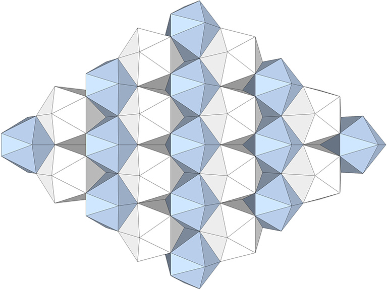
In the jitterbug transformation, the regular icosahedron (white) face-bonds with its space-filling complement (light blue) to form a rhombic lattice.
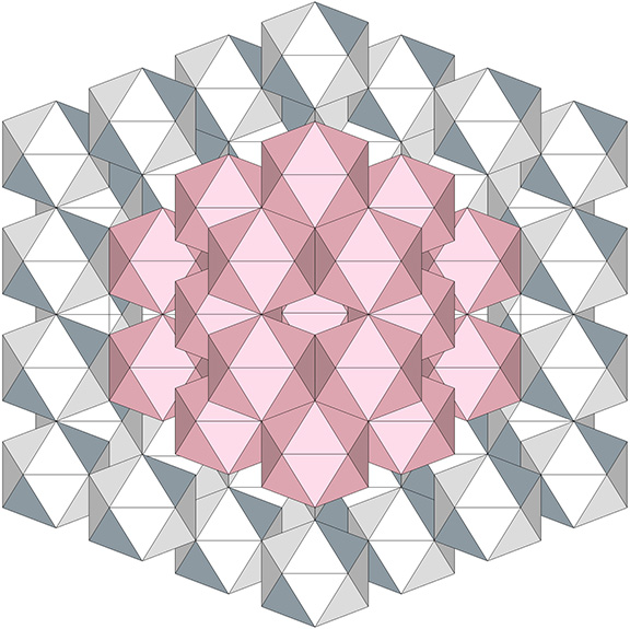
The regular icosahedron and its complement (as well as the Jessen orthogonal icosahedra at tensegrity equilibrium) close pack radially as well as laterally—naturally, as they constitute phases in the jitterbug transformations of the isostropic vector matrix. Note the difference between the close packing of icosahedra as they co-occur in the jitterbug, and the close packing of regular icosahedra around a common center. Here it is 14-around-1, not 12-around-1. Fourteen is the number of faces of the VE, and the number of VEs and octahedra surrounding the central VE in the jitterbugging matrix: six VEs face-bonded to its square faces; plus eight octahedra face-bonded to its triangular faces.
Six regular icosahedra (gray) and eight irregular icosahedra (pink) radially close-pack around a central icosahedron (and vice versa).
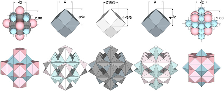
Vector equilibria and octahedra close pack as rhombic dodecahedra that expand and contract during the jitterbug transformation. Maximum expansion coincides with the phase which I call tensor (or tensegrity) equilibrium. It occurs at the precise midpoint of the transformation, when the vector equilibria and octahedra have both transformed into the Jessen orthogonal icosahedron which, not coincidentally, has the same shape as the six-strut tensegrity sphere. (See: Tensegrity.)
The short axis of the rhomboid faces increases from √2 at vector equilibrium, to φ at the icosahedron phases, and to 2√6/3 at tensegrity equilibrium. The long axes increase from 2.0 at vector equilibrium, to φ√2 at the icosahedron phases, and to 4√3/3 at tensegrity equilibrium.
Connecting the centers of the close-packed vector equilibria and octahedra of the isotropic vector matrix describes rhombic dodecahedra that expand and contract during the jitterbug transformation. Spheres exchange places with spaces (top) and vector equilibria exchange places with octahedra (bottom). Maximum expansion occurs at the phase associated with the Jessen orthogonal icosahedron (middle of bottom row.)
The icosahedron and its complement exchange places twice per cycle as the matrix enters and exits tensegrity equilibrium.
The icosahedron and its complement exchange places twice per cycle as the matrix enters and exits tensegrity equilibrium
The angles of the rhombic lattice formed from the regular icosahedron and its complement correspond with the face angles of the rhombic dodecahedron and the dihedral angles of the regular tetrahedron, arctan(√2) and arctan(2√2)) or approximately 54.7356° and 70.5288°.
The rhombic lattice formed from the regular icosahedron and its complement. The rhombus has the same face angles as the rhombic dodecahedron, which are identical to the dihedral angles of the regular tetrahedron.
Regular icosahedra can form icosahedral shells of any frequency, but the shells do not nest inside one another. Note further that the shells do not occur as subdivisions of the lattice. That is, the regular icosahedron may form indefinite lattices or definite shells, but never both in the same matrix.
F2 Icosahedral shell consisting of 42 regular icosahedra, and its concave interior space.
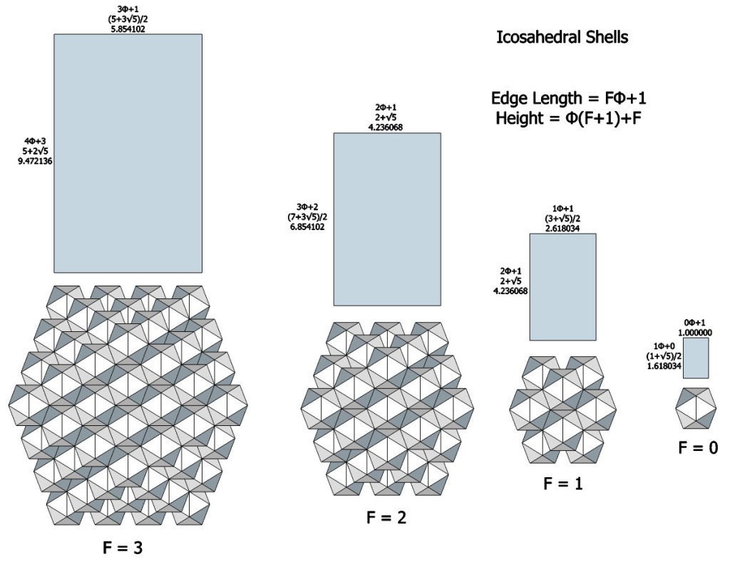
Given icosahedra of unit edge length, the edge length of any icosahedral shell is φ(F)+1, where φ is the golden ratio, (√5+1)/2, and F is the shell frequency. The height of the icosahedron, i.e. the linear dimension of its cubic domain, divided by its edge length is always φ, so the height of any icosahedron shell is φ times its edge length, that is, φ × [φ(F)+1], or φ²F+φ. But since φ²= φ+1, the equation can be rewritten as φ(F+1)+F.
The height times with width of any icosahedral shell is always the golden ratio
Icosahedral shells, F0 through F3, and their dimensions.
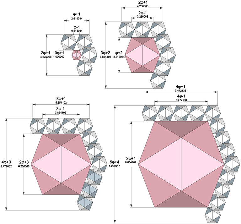
The inside dimensions of the shells follow similar formulas. A regular icosahedron filling the space inside a a shell of frequency F would have the following dimensions:
Note the pattern. The formulas for exterior and interior dimensions differ only by the plus and minus signs.
Exterior and interior dimension of the icosahedral shells, F1 through F4.
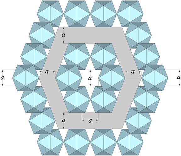
The largest icosahedral shell that can be enclosed within a shell of frequency F has a frequency of F-2. The gap between the two nested shells is always the same of the constituent icosahedron’s edge length. For example, given an edge-length of a for the constituent icosahedra, an F1 shell can fit inside an F3 shell with a gap of a between the F1 shell’s outer surface and the F3 shell’s inner surface.
The gap (a) between the two nested icosahedral shells is always the same of the constituent icosahedron’s edge length.
The F1 shell consists of 12 icosahedra. But if we allow for asymmetry, that is, if we allow the icosahedra to be slid out of alignment and into the cavities between adjacent icosahedra, it is possible to squeeze at least 31 icosahedra inside the F3 shell. The F1 shell is free to rattle around freely inside the F3 shell, but the motion of the 31-icosahedra aggregate seems to be restricted to, at most, just one axis.
if we allow the icosahedra to be slid out of alignment and into the cavities between adjacent icosahedra, it is possible to squeeze at least 31 icosahedra inside the F3 shell.
You can, of course, construct shells from shells, but the resulting shell would have holes. That is, the interior of the larger shell would not be fully isolated from the outside.
F1 Icosahedral shell constructed of twelve F1 icosahedral shells.
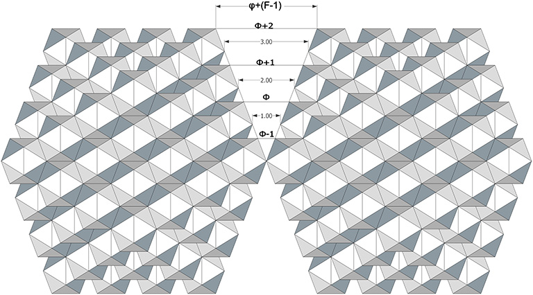
The opening between edge-bonded icosahedral shells is a rhombus whose short diagonal is φ+(F-1).
Gaps between adjacent icosahedral shells follow the formula, φ+(F-1).
The study of icosahedron shells may have implications for and resonance with the behavior of cell membranes and other semi-permeable barriers between systems.
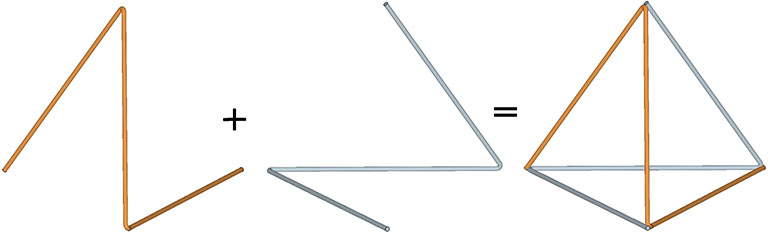
A tetrahedron may be constructed from two open-ended triangles.
Tetrahedron Constructed from Two Open-Ended Triangles
If we use this construction in the isotropic vector matrix, the open ends of each triangle join with similar triangles in the adjacent tetrahedra to form wave patterns that propagate linearly through the matrix, each oriented at 90° to the other. The entire matrix may be built though the duplication of orthogonally paired waves.
Transverse Waves in the Isotropic Vector Matrix
Significant to this model of the isotropic vector matrix is its demonstration of the fundamental principle that no two vectors may pass through the same point simultaneously. All vertices in the matrix redirect their vectors, rather than act as focal points for their convergence.
Deflecting Vectors at Vertices of the Transverse Wave Model of the Isotropic Vector Matrix
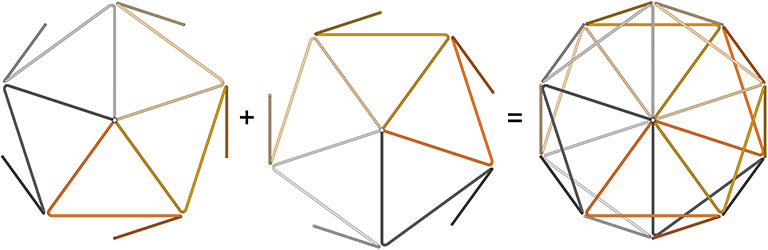
For each of the six axes of the isotropic vector matrix, i.e., the six vertex-to-vertex axes of spin of the vector equilibrium, there are four unique waves, two running clockwise and two running counter clockwise on either side of the axis, for a total of 24 (6×4) waves converging on and deflecting from every point.
For each of the six axes of the isotropic vector matrix, i.e., the six vertex-to-vertex axes of spin of the vector equilibrium, there are four unique waves, two running clockwise and two running counter clockwise on either side of the axis.
Note that the axis that defines the linear orientation of the wave is excluded from the wave itself which traces a path along three of the remaining five edge vectors of the tetrahedron. The clockwise and counter-clockwise waves of the positive and negative tetrahedra each share one leg oriented at 90° to the wave’s directional axis, underscoring the polarization of the pair.
The six axes of the isotropic vector matrix define the six edges of the tetrahedron. The waves from these six axes wrap around each tetrahedron such that each of its six edges includes a leg from four separate waves.
The neutral axes of six chains of open-ended equilateral triangles intersect to form a regular tetrahedron with four vectors per edge.
This recapitulates the quadrivalent (four vectors per edge) tetrahedron that results when the jitterbug is given an extra 180° twist.
With a 180° twist, the jitterbugging VE can be collapsed into a regular tetrahedron with four vectors per edge.
This wave pattern can also be modeled with continuous ribbons of equilateral triangles which are then folded at the same angles as the three vectors of the open-ended triangle above.
The isotropic matrix modeled by the folding of a linear ribbon of equilateral triangles mirrors the transverse wave model of open-ended triangles.
The octahedron can be constructed from four open-ended triangles.
Four open-ended equilateral triangles combine to form the regular octahedron.
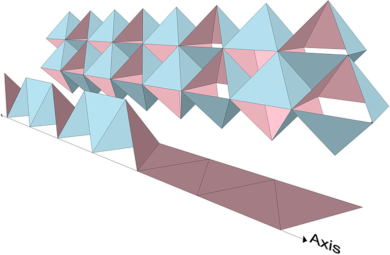
The open-ended triangles of the octahedron may be joined in parallel linear waves that form a continuous chain of octahedra.
The open-ended triangles of the octahedron joined in four parallel linear waves forming a continuous chain of octahedra.
The icosahedron can be constructed from ten open-ended triangles.
Ten open-ended equilateral triangles combine to form the regular icosahedron.
There are numerous ways of joining the open-ended triangles of the icosahedron end-to-end, but all form wave-dispersal patterns in which the icosahedron appears never to repeat.
Joining the open-ended triangles of the regular icosahedron forms a wave-dispersal pattern that appears to never repeat the original icosahedron.
“The geometrical model of energy configurations in synergetics is developed from a symmetrical cluster of spheres, in which each sphere is a model of a field of energy all of whose forces tend to coordinate themselves, shuntingly or pulsatively, and only momentarily in positive or negative asymmetrical patterns relative to, but never congruent with, the eternality of the vector equilibrium. […] Synergetics is comprehensive because it describes instantaneously both the internal and external limit relationships of the sphere or spheres of energetic fields; that is, singularly concentric, or plurally expansive, or propagative and reproductive in all directions, in either spherical or plane geometrical terms and in simple arithmetic.” — R. Buckminster Fuller, Synergetics, 205.01
The point in conventional geometry is replaced by the sphere in Fuller’s geometry. Vertices are the geometric centers of spheres, and vectors connect sphere centers. There are no continuous lines. Surfaces and volumes are point populations, i.e., close-packed spheres or the vertices that define the sphere centers. The minimum point is defined as a vector equilibrium (VE) of zero frequency, i.e. the nuclear sphere. The shell volume of the zero-frequency VE is give by the shell-growth formula for radially close-packed spheres, 10F²+2, as “2,” i.e., the inside surface, plus the outside surface. Unity is plural and at minimum two.
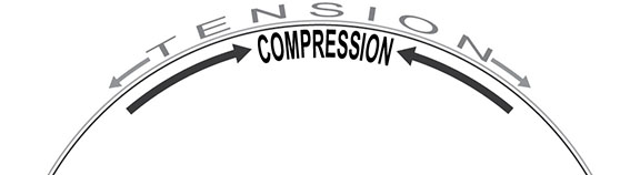
Every sphere has two surfaces, one convex and the other concave. The concave (interior) surface resists compressive forces while the convex (exterior) surface resists tensile forces.
Bending pressure results in tension along the outside of the curve, and compression along the inside of the curve.
In the following illustration, cutaways of the sphere show the concave interior surface (pink) under compression, and the convex exterior surface (blue) under tension.
A sphere holds its shape by balancing the tensile forces of its outer surface (blue) with the compressive forces of it inner surface (pink).
These two forces can be modeled as the radials and circumferential vectors of the vector equilibrium (VE). In the following illustration the radials are represented by rigid struts which resist the compressive force provided by the circumferential vectors represented by elastic bands which in turn resist the tensile force provided by the rigid struts.
The tensile forces of the circumferential vectors of the VE (blue) are balanced by the compressive forces of its radial vectors (brown).
The tensegrity model clearly represents the inter-dependence of the two forces, with the convex tension represented by continuous tendons, and the concave compression represented by the discontinuous struts.
The tensile forces of the 6-strut tensegrity’s continuous tendons are balanced by the compressive forces of its discontinuous struts
In the bow tie model, concave and convex are disclosed as opposite sides of the four great-circle disks that comprise the spherical VE. The combined surface areas of the four disks is the same as the surface area of the sphere they describe. In the illustration below, the two sides are distinguished by color, one pink and the other blue.
In this model of the vector equilibrium (VE), the inside and outside surfaces of the sphere are disclosed as opposite sides of four great-circle disks folded into bow-ties. Their combined surface areas exactly equals the surface ares of the sphere they describe.
In the quanta model, the two forces are represented by the integrative A modules and the dis-integrative B modules. The close packed spheres and spaces which exchange places in the jitterbug, are represented by two rhombic dodecahedra, one being the inside-out version of the other.
The quanta-module construction of the rhombic dodecahedron models the transformation between spheres or spaces in the isotropic vector matrix by turning itself inside out.
The first of the two rhombic dodecahedra has at its core a concave octahedron made entirely of B modules. This core is completely enveloped by A modules, first forming a regular octahedron, and then the rhombic dodecahedron. It suggests an implosive, integrative event.
Quanta module construction of a space.
The second of the two rhombic dodecahedra exposes all of its modules, both A and B, on its surface. None are entirely contained by the others, and it suggests an explosive, dis-integrative event.
Quanta module construction of a sphere.
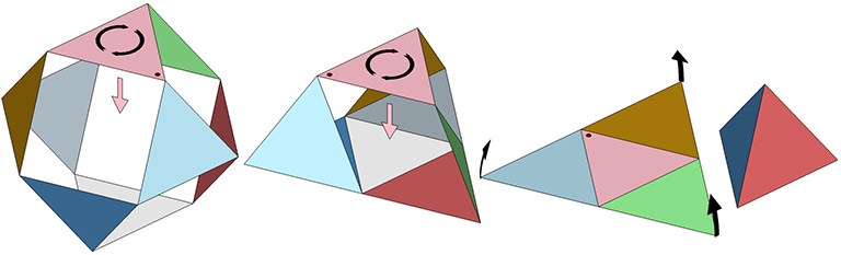
In the jitterbug transformation of the quanta model, the two rhombic dodecahedra exchange places, suggesting one is the explosive space (the expanding octahedron) which takes the place of the imploding nucleus (the contracting VE). This concept may be more clear if we look at the transformations of the core in isolation from the shell.
The core of the the two quanta module constructions of the rhombic dodecahedron. The B quanta modules point outward (sphere) or inward (space).
The B modules are arranged in arrow-like shapes that point their faces inward in the transformation from VE to octahedron (contracting nuclei), and outward in the transformation from octahedron to VE (expanding spaces). Fuller’s intuitions about the energy characteristics of the two modules, entropic for the B quanta modules, syntropic for the A quanta modules, seem all the more inspired the more deeply we look into the geometry.
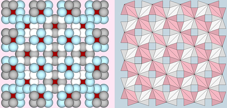
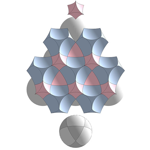
In the interstitial model of the isotropic vector matrix (see Spaces and Spheres Redux), the two forces are made self-evident in the literal exposure of the of the concave interior and convex exterior surfaces of the spheres, represented here as blue concave VE “spaces”, gray convex VE spheres, and pink concave octahedra interstices.
The interstitial model of the isotropic vector matrix exposes the concave inside surfaces of the spheres, as well as the four great circles of the vector equilibrium whose vertices are the points of contact between adjacent spheres.