“The vector equilibrium’s jitterbugging conceptually manifests that any action (and its inherent reaction force) applied to any system always articulates a complex of vector-equilibria, macro-micro jitterbugging, involving all the vector equilibria’s ever cosmically replete complementations by their always co-occurring internal and external octahedra, all of which respond to the action by intertransforming in concert from “space nothingnesses” into closest-packed spherical “somethings,” and vice versa, in a complex threeway shuttle while propagating a total omniradiant wave pulsation operating in unique frequencies that in no-wise interfere with the always omni-co-occurring cosmic gamut of otherly frequenced cosmic vector-equilibria accommodations.“
—R. Buckminster Fuller, Synergetics, 464.06
The Jitterbug is what Fuller called a transformation that occurs when the radial vectors are removed from the otherwise stable configuration of the vector equilibrium (VE).
The whole isotropic vector matrix can be made to jitterbug, with VEs transforming into octahedra, and octahedra into VEs. This coordinated transformation of the isotropic vector matrix suggests a model for omnidirectional wave propagation.
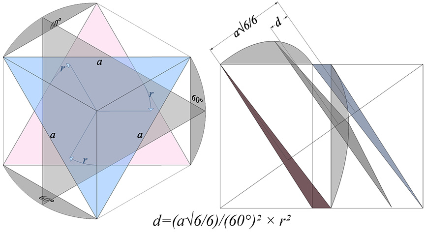
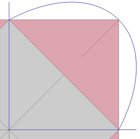
The Jitterbug transformation can be reduced to the rotation of a single triangle inside a cube. If the rotation is constant around the vector described by the cubic diagonal, and the triangle’s vertices are constrained to follow the orthogonal planes defined by the cube as it would in the context of the VE, the triangle will accelerate along the rotation axis. Consequently, the jitterbug seems to “bounce” between phases.
It’s important to note that the oscillations of the jitterbug do not follow a sinusoidal curve, nor do they follow the equations for simple harmonic motion. The formula that almost (see below) seems to work is:
Formula for the jitterbug: d = (√6/6) × a/(60°)² × (r°)²
where a is the edge length of the triangle, and d is the distance traveled along the rotation axis after a rotation of r°.
This parallels the formula for falling objects in a gravitational field:
Formula for a falling object: d=(1/2)×g×t²
We see that (a√6/6)/(60°)² in the jitterbug formula substitutes for the acceleration due to gravity (g) in the formula for falling bodies, and that rotation (r degrees) substitutes for time (t seconds).
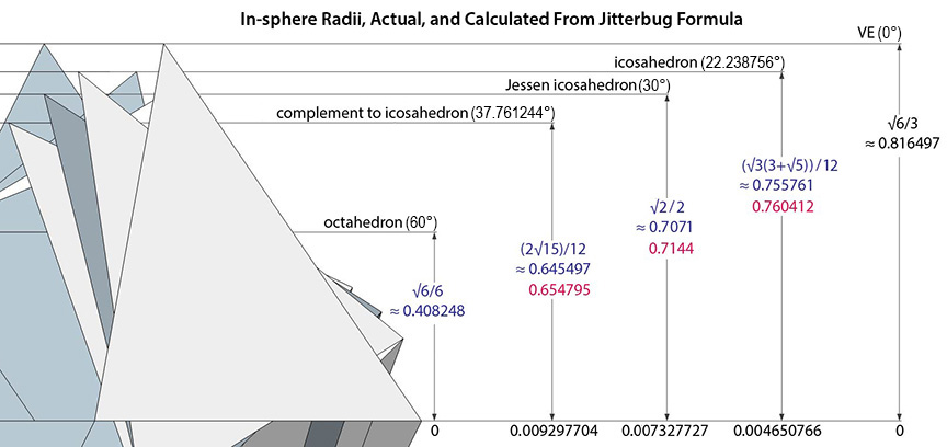
The formula, though adequate for purposes of my illustrations and animations, is not perfect. The in-sphere radii the formula predicts differ from the actual values by as much as 1.4%. For example, the in-sphere radius of the icosahedron (of unit edge-length) is φ²√3/6 ≈ 0.755761, while the formula calculates a value of approximately 0.760412, a difference of about 0.00465. The in-sphere radii of the Jessen icosahedron, and the space-filling complement to the regular icosahedron are √2/2 ≈ 0.7071 and 2√15/12 ≈ 0.645497, respectively. The formula calculates values of 0.7144 and 0.654795, a difference of about 0.00733 and 0.00930 respectively.
The arc described by the triangle’s vertices follow what appears to be a hyperbolic path. Fuller assumed the path should be a geodesic arc describing a spherical cube. I find the actual hyperbolic shape more intriguing, however, as it suggests a four-dimensional geodesic, e.g., the swing-by trajectory of an object passing through a gravitational field.
Approximately midway between the vector-equilibrium and octahedron phases, the jitterbug describes the regular icosahedron. The collapsing VEs and expanding octahedra, however, do not simultaneously describe the regular icosahedron. The common shape, precisely midway between the transformation from one to the other, is actually the shape of the six-strut tensegrity sphere. Fuller neglected to give the shape a name, perhaps failing to appreciate its full significance. Other mathematicians, namely Borge Jessen, have taken credit for its “discovery,” and Wikipedia affirms its identity as the Jessen Orthogonal Icosahedron.
In the figure below, the Jessen orthogonal icosahedron is on the far right. The others are variations of the tensegrity model, all of which match its shape exactly.
See also: Icosahedron Phases of the Jitterbug.
Any two parallel struts of the six-strut tensegrity sphere can be alternately pulled outward and pushed inward to recapitulate the jitterbug of the vector model.
If we allow the edges of the triangles to shorten and lengthen as they do with the expansion and contraction of the 6-strut tensegrity sphere, the jitterbug should oscillate like a pendulum or guitar string, rather than a bouncing ball.
The VE may be conceived as eight regular tetrahedra sharing a common vertex, and the jitterbug as the oscillation between positive and negative tetrahedra. See The Dual Nature of the Tetrahedron.
The operation is made more explicit, I think, in another tensegrity model of the jitterbug which focuses on the eight tetrahedra rather than the VE. The six-strut tensegrity sphere can be transformed, through coordinated clockwise or counter-clockwise rotations of the struts, into either a positive or negative tetrahedron.
The two tensegrity models of the jitterbug can be placed one inside the other with surprisingly little or no interference. This may be the truest model of the jitterbug transformation as the natural state of the isotropic vector matrix. In the vector model, the transformation is instigated by the removal of the twelve radial vectors from the VE, whereas in this and the following models, its only trigger is the spontaneous reversal of the tetrahedra; no quanta are lost or created in the process.
For more information on transformational operations of the six-strut tensegrity sphere, as well as the twelve- and thirty-strut tensegrity spheres, see Tensegrity.
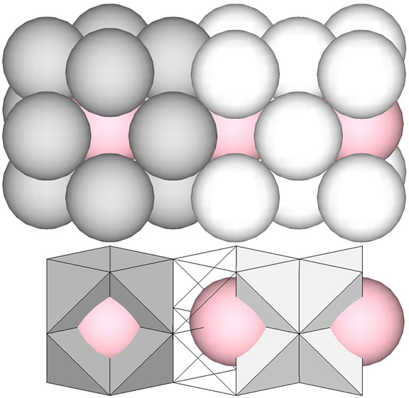
In the interstices model (See Spaces and Spheres, and Spaces and Spheres (Redux)), the eight tetrahedra occupy the interstices (concave octahedra) between close-packed spheres. The VE phase defines the nuclear domain, and the octahedron phase defines the space (a concave VE) left by the removal, transformation, or collapse, of the nucleus. This model emphasizes the space-to-sphere, sphere-to-space oscillations of jitterbug. Note that the interstices, i.e., the eight tetrahedra defining the the concave octahedra, are the only constant in the jitterbug; the spheres and spaces (VEs and octahedra) emerge as a consequence of the positive-negative oscillations of the tetrahedra.
The quanta model elegantly recapitulates the sphere-to-space, space-to-sphere transformation with the two quanta module constructions of the rhombic dodecahedron:
When modeled with spheres, the isotropic vector matrix divides naturally into cubic and VE modules. The cubic modules consist of 14 spheres, one more than VE’s 13, i.e., 12 spheres around a central nuclear sphere.
This suggests a model for the jitterbug in which the nuclei migrate between cubes and the VEs.
For further discussion of the sphere-to-space, space-to-sphere oscillations of the jitterbug, see: Quanta Module Constructions of the Rhombic Dodecahedron; and Great Circle Bow-Ties of the VE.
