“The XYZ-rectilinear coordinate system of humans fails to accommodate any finite resolution of any physically experienced challenge to comprehension. Physical experience demonstrates that individual-unit wavelength or frequency events close-pack in spherical agglomerations of unit radius spheres.”
—R. Buckminster Fuller, Synergetics, 260.31
Unit-radius spheres close pack in three fundamentally different ways:
- radially around a central nucleus to form the isotropic vector matrix;
- laterally as discrete icosahedron shells and lattices (see The Icosahedron; and Close Packing of Icosahedra), and;
- linearly as discrete triple helices of face-bonded tetrahedra (see Tetrahelix).
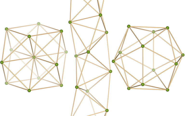
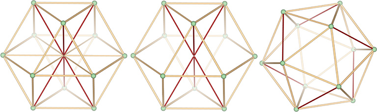
The relative stability of these arrangements is perhaps made more clear when modeled with unit-length sticks, representing the vectors connecting sphere centers, and flexible connectors. The radial array on the left is the vector equilibrium (VE) and isotropic vector matrix; the linear array in the middle is the tetrahelix; and the lateral array on the right is the icosahedral shell.
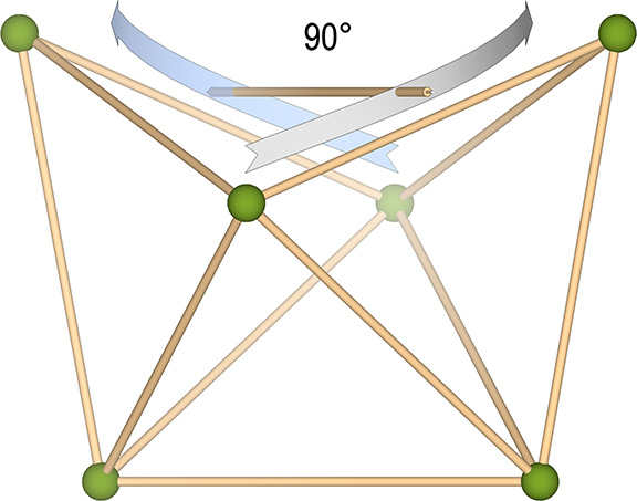
The transformation between the isotropic radial array and the linear (helical) array can be described as three face-bonded tetrahedra transforming into a single octahedron.
The structural transformation is more clearly illustrated with a vector model.
Fuller thought this transformation modeled quantum energy dispersion and absorption, with the three-tetrahedron array gaining one quantum of energy in the transformation to the octahedron, which has volume for four (3+1) tetrahedra. Likewise, the octahedron loses one quantum in the transformation from a volume of four to the volume of three tetrahedra.
Note that the transformation involves the 90° rotation of one of the struts. Fuller would identify this as an example of “precession” about which he had much to say. It occurred to him that whenever energy is gained, lost, or otherwise transformed by a system, precession is always involved, and is geometrically manifested in effects at 90° to the perceived action.
The transformation between the radial and the lateral can be described as the transformation that occurs when the nuclear sphere is removed from the VE configuration. The twelve remaining spheres then rearrange themselves into an icosahedron.
The VE twists to the right or to the left to form a positive or a negative icosahedron. Note that this effect, too, is precessional, i.e., the gain and loss of energy is accompanied by a circumferential effect that is at 90° to the radial disappearance of the nucleus. In the vector model, the loss of the nucleus is presented as the disappearance of six of the VE’s twelve radial vectors. Six vectors equals one tetrahedron, or one quantum of energy. The remaining six radial vectors are added to the 24 edge vectors of the VE to compose the 30-edge, structurally stable icosahedron.
It’s important to remember, however, that the energy is only displaced, not destroyed. When the transformation is reversed, the six radial vectors are reintegrated, not created. This is more clearly demonstrated in the jitterbugging of the isotropic vector matrix, of which this transformation is an isolated part.
The isotropic vector matrix produces close packed arrays not only of vector equilibria, but also of tetrahedra, octahedra, cubes, rhombic dodecahedra, as well as other polyhedra. However, only the VE construction has uniform and uninterrupted shell growth around a single nuclear sphere. Other polyhedra cluster around the nucleus in either every other layer, as is the case with spheres close-packed as octahedra, or in every fourth layer, as is the case with spheres close packed as tetrahedra or cubes.
Equations for the Close Packing of Spheres
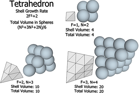
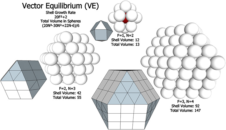
For the shell growth rate in spheres, F is the number of subdivisions along any one edge. That is, you count the spaces between the spheres rather than the spheres themselves. For total sphere volume, N is the number of spheres along any one edge. That is N = F+1.
Shell Growth Rates
The shell growth rate formulas all follow the same pattern, nF²+2.
- Tetrahedron: 2F2+2
- Octahedron: 4F2+2
- Cube: 3F²+2 (even layers), or 3F²+1 (odd layers)*; 6F²+2**
- Vector Equilibrium (VE): 10F2+2
- Rhombic Dodecahedron: 12F²+2***
* Spheres close-packed as cubes in the 60° grid of the isotropic vector matrix will have a shell volume of 3F²+2 in even-numbered layers only. Odd-numbered layers produce cubes with four truncated corners, and its formula is 3F²+1.
** Spheres stacked as cubes on the 90° grid will have a shell volume of 6F²+2, but the configuration is unstable.
*** Spheres stacked as rhombic dodecahedra on a rhomboid grid will have a shell volume of 12F²+2, but the configuration is unstable. Spheres close-packed as rhombic dodecahedra in the the isotropic vector matrix are defined by close-packed nuclear domains rather than the spheres themselves. See Formation and Distribution of Nuclei in Radial Close-Packing of Spheres.
Total Number of Spheres
- Equilateral Triangle: [(F+1)²+(F+1)]/2
- Tetrahedron: [(F+2)³-(F+2)]/6
- Half Octahedron: (2F³+9F²+13F+6)/6
- Octahedron: [4(F+1)³+2(F+1)]/6
- Vector Equilibrium: (20F³+30F²+22F+6)/6
- Equilateral Triangle: (N²+N)/2 = (3N²+3N)/6
- Tetrahedron: [(N+1)³-(N+1)]/6 = (N³+3N²+2N)/6 = (F³+6F²+11F+6)/6
- Half Octahedron: N(N+1)(2N+1)/6 = (2N³+3N²+N)/6
- Octahedron: 2N(2N²+1)/6 = (4N³+2N)/6
- Vector Equilibrium: (20N³-30N²+22N-6)/6

The excess “two” in the shell growth rates also appears in the topological abundance formulas. See also: The Multiplicative and Additive Two; and Concentric Sphere Shell Growth Rates.
