If a spherical nucleus were at the center of a close-packed array of spheres in the icosahedron configuration, what would be its radius? That is, by how much must the nucleus shrink when the close-packed array jitterbugs from the VE to the icosahedron? Knowing that the icosahedron can be constructed from the three golden rectangles arranged orthogonally around a common center, it’s a simple matter of trigonometry.
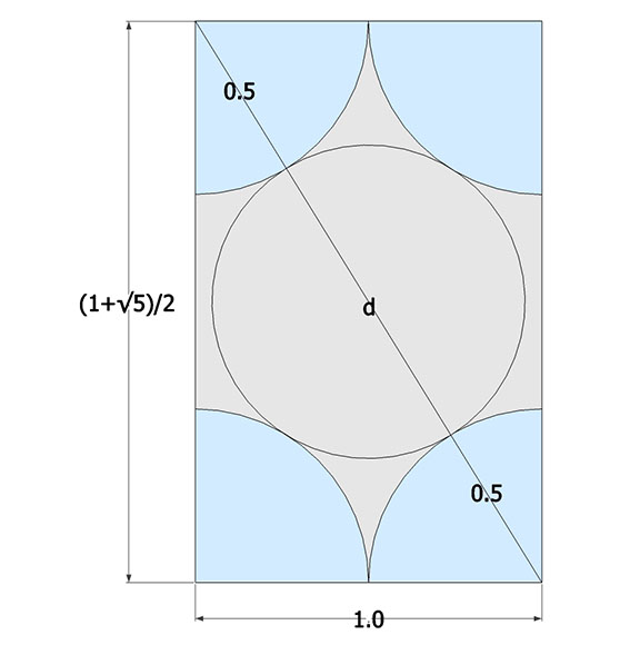
The regular icosahedron can be constructed from three intersecting golden rectangles.
The diagonal, d, of the regular icosahedron is equal to the diagonal of the golden rectangle from which it is constructed. The diameter for the center circle is d-1.
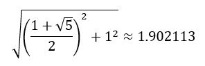
The diagonal (d) is the the square root of the sum of the squares of the two sides, or √(((1+√5)/2)+1²) ≈ 1.902113:
The diameter of the nucleus at the center of an icosahedron made up of unit-radius spheres is the length of the diagonal minus 1, or approximately 0.902113.
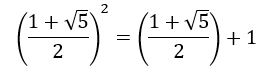
The golden ratio has some curious properties. For example, its square is equal to itself plus one:
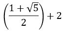
Knowing this, we can reduce the expression under the radical above to ((1+√5)/2)+2:
Since the expression on the left is the golden ratio, it follows that the diagonal of the icosahedron may be expressed as √(2+φ):
The isotropic vector matrix can be modeled as vectors, struts and tendons, quanta modules, or as spheres and their interstices. All these models originated in Fuller’s geometry with the close packing of unit-radius spheres—ping-pong balls or Styrofoam spheres he glued together. We may be tempted to think of these spheres, as we used to the think of atoms, as solid and indivisible. But by now we should be accustomed to thinking of these fundamental particles as divisible into obscure quanta with strange properties, as clouds of energy, or as waves in a quantum field. So it may not bother us to see these otherwise solid spheres merging and diverging in the spherical model of the jitterbug.
The jitterbug as a single VE with its vertices represented by unit spheres.
But if we think of the spheres as quanta, their number, by fundamental conservation laws, should remain constant throughout the jitterbug. If we assume one sphere per vertex, what is the ratio of vertices in the isotropic vector matrix compared to the matrix at tensegrity equilibrium? The former includes the nuclei which are replaced by the six struts in the tensegrity model. But it does not appear that those make up for the increase in the number of vertices, i.e. shell vertices plus nuclei in the vector model do not add up to the number of vertices in the tensegrity model. Where do the extra spheres/vertices come from?
Fuller thought the vectors, whose length defines the sphere diameter, were a constant in the jitterbug. But it appears that the true constant in the jitterbug is the length of the diagonal, i.e. the length of the struts in the tensegrity model. If we hold the strut length constant, the spheres do not fully divide in the icosahedron phases of the jitterbug. When the jitterbug is conceived as an unbounded matrix, the spheres never divide without simultaneously merging with neighboring spheres (which are also dividing).
The partial division of the spheres that reaches its maximum at the Jessen phase, i.e., at tensegrity equilibrium, might be conceived as the counterpart to the separation of tension and compression in the tensegrity model. That is, the spheres’ convexity (tension) and concavity (compression) are being isolated in the same way that the tendons (tension) and struts (compression) are isolated in the tensegrity model.
The jitterbug, oscillating into and out of tensegrity equilibrium. Note that maximum division of the spheres occurs between, not at, the vector equilibrium phases.
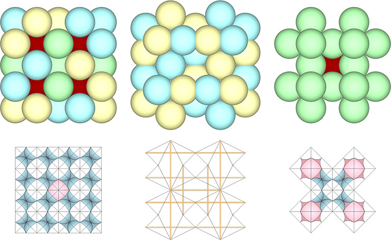
In the figure below, this division of spheres into the convex and concave counterparts is represented by green spheres dividing (partially) into blue and yellow spheres, and then recombining into green spheres.
Three phases of the jitterbug represented as unit spheres (top), as spaces and interstices (bottom left and right), and by six-strut tensegrity spheres (bottom middle). The green spheres partially divide into blue and yellow spheres in the icosahedron phases of the jitterbug (top middle. Each blue-yellow pair constitutes one sphere.
Isotropy is restored when the VE contracts into an octahedron and when the octahedron expands to the VE. But in between, when both shapes describe regular or irregular icosahedra, the only constant is the strut length which (if the vectors at equilibrium are of unit length) is equal to √2, the diagonal of the unit-edged cube.
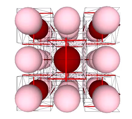
The increase in the number of vertices is modeled in the tensegrity model of the jitterbug as the merging and diverging of struts. The struts, like the spheres, are doubled up at vector equilibrium, and do not quite fully separate at tensegrity equilibrium. In the figure below, the nuclei in the sphere model have been superimposed onto the tensegrity matrix at vector equilibrium. The red nuclei are associated with 12-sphere shells unique to that nucleus. The pink nuclei share their 12-sphere shells with the surrounding nuclei. (See Formation and Distribution of Nuclei in Radial Close-Packing of Spheres.)
The distribution of nuclei superimposed onto the tensegrity model at vector equilibrium.
To see how the struts in the tensegrity model serve the same purpose as the nuclei in the sphere model, imagine the tensegrity jitterbug with the struts squeezed together into the octahedron configuration. As the struts separate, imagine unit-radius spheres centered at each of their ends. They start out as porous clouds but harden into impenetrable spheres just as the struts have separated into the VE configuration. The tensegrity-plus-spheres model is at equilibrium, with the spheres and struts both supplying compression resistance to the tension web of tendons. The de-nucleated sphere shell will not collapse into an icosahedron as long as the struts remain rigid.
The tensegrity model at vector equilibrium, when coupled with the spheres model, holds the spheres in the same 12-around-1 configuration as radially close-packed spheres around a common nucleus.
This model underscores Fuller’s proposition that gravity is a 90° precessional effect. That is, mass-attraction is modeled here by the tension web, the chords between the sphere centers which are situated at right angles to the radial vectors which would otherwise connect each to their common nucleus. The nucleus of the radially close-packed spheres model has here been replaced with the struts of the tensegrity model.